Lecture 19: Least squares fitting

Lecture 19: Least squares fitting#

Motivation#

Suppose we are given data point representing a quantity over time.
We want to represent the graph of this data as a simple curve.
The examples on the following slide show the fitting of two different curves through some experimental data:
- a straight line;
- a quadratic curve.

Weekly earnings#

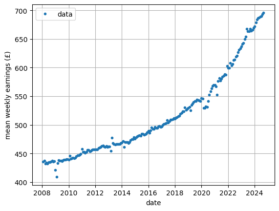
Raw data for weekly earnings:

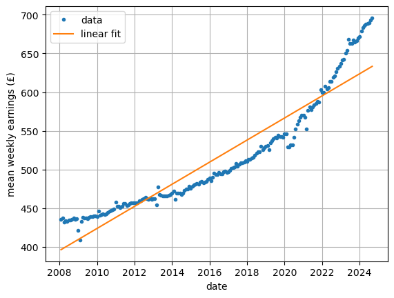
../_images/2ec147b3a412db78b6d22f25dbde1cd891b19358cd31eb138fef83f1f2bdc75d.png

Raw data for weekly earning with a straight line of best fit:

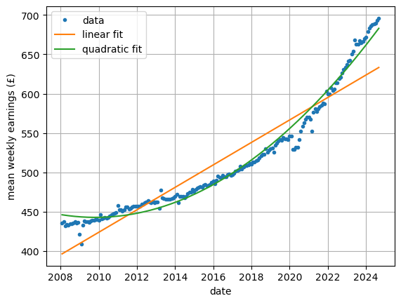
../_images/40f117f7c089990f59899af892b1ef051d56b672169dbe850de757e1c0a6788f.png

Raw data for weekly earnings with a quadric curve of best fit:

../_images/2ecff142d11c3ef304036afd445c6500eb0df681ad8f0337e23bce4b147ae411.png

Data source, ons, [xls]

An example of best linear fit#

Suppose that the following measured data, \(y\), is observed at different times \(t\):

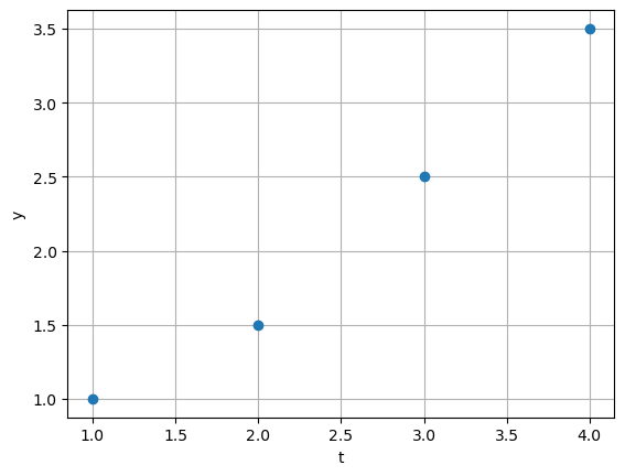
\[\begin{split} \begin{array}{c|cccc} t & 1 & 2 & 3 & 4 \\ \hline y & 1 & 1.5 & 2.5 & 3.5 \end{array} \end{split}\]

../_images/676910153a7a16d18b7117443d09ad6985d869158ce8de9e035512ba29018efd.png

Consider representing this data as a straight line:

\[ y = mt + c \]
An exact fit would require the following equations to be satisfied:

\[\begin{split} \begin{aligned} m \times 1 + c & = 1 \\ m \times 2 + c & = 1.5 \\ m \times 3 + c & = 2.5 \\ m \times 4 + c & = 3.5. \end{aligned} \end{split}\]

We recognise this as a system of linear equations for \((m, c)\) - but there are too many equations!!

An example of best quadratic fit#

Suppose that the following measured data, \(y\), is observed at different times \(t\):

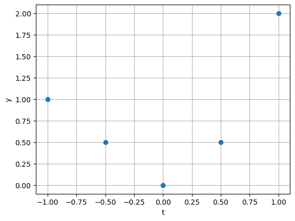
\[\begin{split} \begin{array}{c|ccccc} t & -1.0 & -0.5 & 0 & 0.5 & 1.0 \\ \hline y & 1.0 & 0.5 & 0.0 & 0.5 & 2.0 \end{array} \end{split}\]

../_images/d05fac1bd7012ec4152164ae58f09d67e7630d1eda9dd67454a52d46189617e6.png

Consider representing this data as a quadratic line:

\[ y = a + b t + c t^2 \]
An exact fit would require the following equations to be satisfied:

\[\begin{split} \begin{aligned} a + b \times -1 + c \times (-1)^2 & = 1 \\ a + b \times -0.5 + c \times (-0.5)^2 & = 0.5 \\ a + b \times 0 + c \times 0^2 & = 0 \\ a + b \times 0.5 + c \times 0.5^2 & = 0.5 \\ a + b \times 1 + c \times 1^2 & = 2. \end{aligned} \end{split}\]

We recognise this as a system of linear equations for \((a, b, c)\) - but there are too many equations!!

Best approximation#

Given that there is no exact fit solution to these overdetermined systems of equations what should we do?
Recall the definition of the residual for the system \(A \vec{x} = \vec{b}\):

\[ \vec{r} = \vec{b} - A \vec{x}, \]
- When \(\vec{r} = \vec{0}\), then \(\vec{x} = \vec{x}^*\) the exact solution.
- When there is no exact solution the next best thing is to make \(\vec{r}\) as small as possible.
- This means finding \(\vec{x}\) that minimises \(\| \vec{r} \|^2\).

The normal equations#

It turns out that the \(\vec{x}\) that minimises \(\| \vec{b} - A \vec{x} \|^2\) is the same \(\vec{x}\) that satisfies that following square systems of equations:

\[ A^T A \vec{x} = A^T \vec{b}. \]

These equations are referred to as the normal equations for the overdetermined system \(A \vec{x} = \vec{b}\).
The square matrix \(A^T A\) is generally non-singular (i.e., the solution is unique).
You can find this solution using Gaussian elimination (for example).
The normal equations, when solved, give the best solution to the original problem in the sense of minimising the Euclidean norm of the residual.

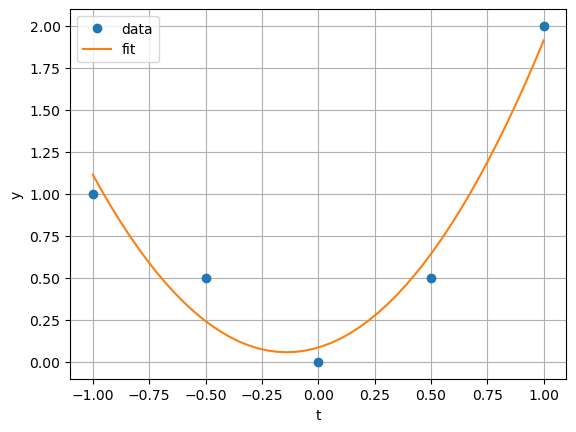
Example I#

Find the least squares approximation to the quadratic fit example.

The residual is given by

\[\begin{split} \begin{aligned} \vec{r} & = \vec{b} - A \vec{x} \\ & = \begin{pmatrix} 1 \\ 0.5 \\ 0 \\ 0.5 \\ 2 \end{pmatrix} - \begin{pmatrix} 1 & -1 & 1 \\ 1 & -0.5 & 0.25 \\ 1 & 0 & 0 \\ 1 & 0.5 & 0.25 \\ 1 & 1 & 1 \end{pmatrix} \begin{pmatrix} x_1 \\ x_2 \\ x_3 \end{pmatrix} \end{aligned} \end{split}\]

We want to find \(\vec{x}\) that minimises

\[ \| \vec{r} \|^2 = \| \vec{b} - A \vec{x} \|^2. \]

The left and right hand sides of the normal equations are given by

\[\begin{split} \begin{aligned} A^T A & = \begin{pmatrix} 1 & 1 & 1 & 1 & 1 \\ -1 & -0.5 & 0 & 0.5 & 1 \\ 1 & 0.25 & 0 & 0.25 & 1 \end{pmatrix} \begin{pmatrix} 1 & -1 & 1 \\ 1 & -0.5 & 0.25 \\ 1 & 0 & 0 \\ 1 & 0.5 & 0.25 \\ 1 & 1 & 1 \end{pmatrix} \\ & = \begin{pmatrix} 5 & 0 & 2.5 \\ 0 & 2.5 & 0 \\ 2.5 & 0 & 2.125 \end{pmatrix} \end{aligned} \end{split}\]

and

\[\begin{split} A^T \vec{b} = \begin{pmatrix} 1 & 1 & 1 & 1 & 1 \\ -1 & -0.5 & 0 & 0.5 & 1 \\ 1 & 0.25 & 0 & 0.25 & 1 \end{pmatrix} \begin{pmatrix} 1 \\ 0.5 \\ 0 \\ 0.5 \\ 2 \end{pmatrix} = \begin{pmatrix} 4 \\ 1 \\ 3.25 \end{pmatrix} \end{split}\]

We can apply Gaussian elimination to solve this problem (only one row operation is required!). The algorithm gives:

\[\begin{split} \begin{pmatrix} 5 & 0 & 2.5 \\ 0 & 2.5 & 0 \\ 0 & 0 & 0.875 \\ \end{pmatrix} \begin{pmatrix} x_1 \\ x_2 \\ x_3 \end{pmatrix} = \begin{pmatrix} 4 \\ 1 \\ 1.25 \end{pmatrix}, \end{split}\]

and backward substitution gives (to 4 significant figures)

\[ \vec{x} = (0.08571, 0.4000, 1.429). \]

../_images/2d48dcbc4d7cb265018a2c38e403638ee0c4f932b8d0b55aef882cda004bbdfe.png

Example 2 (homework)#

Find the least square approximation to the system given by

\[\begin{split} \begin{pmatrix} -2 & 2 & -1 \\ 0 & 1 & 0 \\ 3 & 1 & -2 \\ 1 & 1 & 4 \end{pmatrix} \begin{pmatrix} x_1 \\ x_2 \\ x_3 \end{pmatrix} = \begin{pmatrix} 2 \\ 1 \\ 0 \\ -3 \end{pmatrix} \end{split}\]

Problems with the normal equations#

Consider the matrix \(A = \begin{pmatrix} 1 & 1 \\ \varepsilon & 0 \\ 0 & \varepsilon \end{pmatrix}\), which gives

\[\begin{split} A^T A = \begin{pmatrix} 1 + \varepsilon^2 & 1 \\ 1 & 1 + \varepsilon^2. \end{pmatrix} \end{split}\]

If \(\varepsilon \approx \sqrt{eps}\) then the effects of rounding error can make \(A^T A\) appear to be singular.

See also: Nick Higham, Seven sins of numerical linear algebra

Sensitivity and conditioning#

The condition number of a square matrix \(A\) describes how close that matrix is to being singular.
If the condition number is larger then \(A\) is “close” to being singular.
When the condition number is very large it is likely that the effects of rounding errors will be most serious: we refer to such a system as being ill-conditioned.
The normal equations are typically quite ill-conditioned and so it is essential to use high precision arithmetic to solve them and specialised algorithms.

Summary#

Overdetermined systems are common in data modelling and they typically have no solution.
Even so, it is possible to find a closest solution to the problem.
It is common to measure this closeness in the Euclidean norm and this leads naturally to the least squares approximation.
A solution to this problem can be found by solving the normal equations but can must be taken to use arithmetic with sufficient precision and specialised algorithms.