Lecture 13: Exact solutions and errors#
Exact derivatives and exact solutions#
In some special cases it is possible to evaluate the derivative of a function exactly.
Similarly, in some special cases it is possible to solve a differential equation exactly.
In general, however, this is not the case and so numerical methods are required - this is what this module is concerned with.
The special, exact, cases are not what this module is about, however it is helpful to consider one or two examples.
Example 1#
Consider the function \(y(t) = t^2\).
We can plot an estimate of the graph of \(y'(t)\) quite easily in this case:
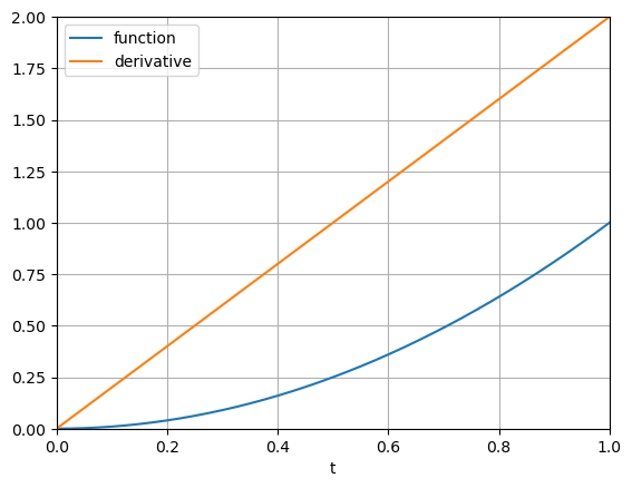
In fact we may use the definition of \(y'(t)\) to evaluate this function at any point:
\[ y'(t) = \lim_{\mathrm{d}t \to 0} \frac{y(t + \mathrm{d}t) - y(t)}{\mathrm{d}t}. \]When \(y(t) = t^2\) we know that
\[\begin{split} \begin{aligned} \frac{y(t + \mathrm{d}t) - y(t)}{\mathrm{d}t} & = \frac{(t + \mathrm{d}t)^2 - t^2}{\mathrm{d}t} \\ & = \frac{t^2 + 2 \times t \times \mathrm{d}t + ( \mathrm{d}t )^2 - t^2}{\mathrm{d}t} \\ & = 2 t + \mathrm{d}t. \end{aligned} \end{split}\]Taking the limit \(\mathrm{d}t \to 0\), we see that \(y'(t) = 2t\).
Example 2#
Similarly, when \(y(t) = t^3\) we have
\[\begin{split} \begin{aligned} \frac{y(t + \mathrm{d}t) - y(t)}{\mathrm{d}t} & = \frac{(t + \mathrm{d}t)^3 - t^3}{\mathrm{d}t} \\ & = \frac{t^3 + 3 \times t^2 \times \mathrm{d}t + 3 \times t \times (\mathrm{d}t)^2 + (\mathrm{d}t)^2 - t^3}{\mathrm{d}t} \\ & = 3 \times t^2 + 3 \times t \times \mathrm{d}t + (\mathrm{d}t)^2. \end{aligned} \end{split}\]Now taking the limit as \(\mathrm{d}t \to 0\) we see that, in this case \(y'(t) = 3t^2\).
In general, we may show that when \(y(t) = t^m\), then \(y'(t) = m t^{m-1}\).
Example 3#
By working backwards from a known expression for \(y(t)\) and \(y'(t)\) we can make up our own differential equation that has \(y(t)\) as a known solution.
e.g., when \(y(t) = t^3\):
\[ y'(t) = 3 t^2 = 3y(t) / t. \]Hence we know the solution to the following equation:
\[ y'(t) = 3 y(t) / t \quad \text{ subject to } \quad y(1) = 1. \]If we solve this for values of \(t\) between \(1.0\) and \(2.0\), say, then we know that exact answer when \(t = 2.0\) is \(y(2) = 8\).
Errors in Euler’s method#
We can solve this problem using Euler’s method and then look at the errors when \(t = 2.0\).
| n | dt | solution | abs. error | ratio |
|---|---|---|---|---|
| 10 | 0.100000 | 7.000000 | 1.000000 | --- |
| 20 | 0.050000 | 7.454545 | 0.545455 | 0.545455 |
| 40 | 0.025000 | 7.714286 | 0.285714 | 0.523810 |
| 80 | 0.012500 | 7.853659 | 0.146341 | 0.512195 |
| 160 | 0.006250 | 7.925926 | 0.074074 | 0.506173 |
| 320 | 0.003125 | 7.962733 | 0.037267 | 0.503106 |
| 640 | 0.001563 | 7.981308 | 0.018692 | 0.501558 |
What is happening to the error as \(\mathrm{d}t \to 0\)?
It is decreasing
Each time \(\mathrm{d}t\) is halved the error is halved.
The error is proportional to \(\mathrm{d}t\).
What might we expect the computed solution to be if we halved \(\mathrm{d}t\) one more time?
Big O Notation#
In considering algorithm complexity you have already seen this notation. For example:
Gaussian elimination requires \(O(n^3)\) operations when \(n\) is large.
Backward substitution requires \(O(n^2)\) operations when \(n\) is large.
For large values of \(n\) the highest powers of \(n\) are the most significant.
For smaller values of \(\mathrm{d}t\), it is the lowest powers of \(\mathrm{d}t\) that are the most significant:
when \(\mathrm{d}t = 0.001\), \(\mathrm{d}t\) is much bigger than \((\mathrm{d}t)^2\) for example.
We can make use of the “big O” notation in either case.
For example, suppose \(f(x) = 2 x^2 + 4 x^3 + x^5 + 2 x^6,\)
then \(f(x) = O(x^6)\) as \(x \to \infty\)
and \(f(x) = O(x^2)\) as \(x \to 0\).
In this notation, we can say that the error in Euler’s method is \(O(\mathrm{d}t)\).
Improving upon Euler’s method#
Let’s assume that the error in Euler’s method is proportional to \(\mathrm{d}t\).
Then halving \(\mathrm{d}t\) will halve the error.
Suppose the error in taking one step of size \(\mathrm{d}t\) is \(E\), call this solution \(\alpha\), then taking two steps of size \(\frac{1}{2} \mathrm{d}t\) should yield and error of \(E/2\), call this solution \(\beta\):
\[\begin{split} \begin{aligned} \alpha - y_{\text{exact}} &= E \\ \beta - y_{\text{exact}} &= E/2. \end{aligned} \end{split}\]Subtracting twice the second equation from the first gives:
\[ y_{\text{exact}} = 2 \beta - \alpha, \]which should be an improved approximation.
We use this idea to derive a improve numerical scheme.
The midpoint scheme#
To get \(\alpha\) take a single step of size \(\mathrm{d}t\):
\[ \alpha = y^{(i)} + \mathrm{d}t f(t^{(i)}, y^{(i)}). \]To get \(\beta\) take two steps of size \(\mathrm{d}t/2\):
\[\begin{split} \begin{aligned} k & = y^{(i)} + (\mathrm{d}t / 2) f(t^{(i)}, y^{(i)}) \\ m & = t^{(i)} + \mathrm{d}t / 2 \\ \beta & = k + (\mathrm{d}t / 2) f(m, k). \end{aligned} \end{split}\]Combining \(\alpha\) and \(\beta\) as suggested the slide before last gives
\[\begin{split} \begin{aligned} y^{(i+1)} & = 2 \beta - \alpha \\ & = 2 (k + (\mathrm{d}t/2) f(m, k) )- (y^{(i)} + \mathrm{d}t f(t^{(i)}, y^{(i)})) && \text{(sub for $\alpha$ and $\beta$)} \\ & = 2 k - y^{(i)} + \mathrm{d}t (f(m, k) - f(t^{(i)}, y^{(i)})) && \text{(rearrange)} \\ & = 2 (y^{(i)} + (\mathrm{d}t / 2) f(t^{(i)}, y^{(i)})) - y^{(i)} \\ & \qquad + \mathrm{d}t (f(m, k) - f(t^{(i)}, y^{(i)})) && \text{(sub for $k$)} \\ & = y^{(i)} + \mathrm{d}t f(m, k) && \text{(rearrange and cancel terms)}. \end{aligned} \end{split}\]As a computational algorithm this gives an algorithm:
Initialise starting values \(t^{(0)}\) and \(y^{(0)}\).
Loop over all time steps, until the final time, updating using the formulae:
\[\begin{split} \begin{aligned} k & = y^{(i)} + (\mathrm{d}t / 2) f(t^{(i)}, y^{(i)}) \\ m & = t^{(i)} + \mathrm{d}t / 2 \\ y^{(i+1)} & = y^{(i)} + \mathrm{d}t f(m, k) \\ t^{(i+1)} & = t^{(i)} + \mathrm{d}t. \end{aligned} \end{split}\]for i in range(n): y_mid = y[i] + 0.5 * dt * f(t[i], y[i]) t_mid = t[i] + 0.5 * dt y[i+1] = y[i] + dt * f(t_mid, y_mid) t[i+1] = t[i] + dt
Results#
The following tables shows computed results for the final solution, at \(t = 2.0\).
| n | dt | solution | abs. error | ratio |
|---|---|---|---|---|
| 10 | 0.100000 | 7.935060 | 0.064940 | --- |
| 20 | 0.050000 | 7.982538 | 0.017462 | 0.268892 |
| 40 | 0.025000 | 7.995475 | 0.004525 | 0.259127 |
| 80 | 0.012500 | 7.998849 | 0.001151 | 0.254473 |
| 160 | 0.006250 | 7.999710 | 0.000290 | 0.252212 |
| 320 | 0.003125 | 7.999927 | 0.000073 | 0.251100 |
| 640 | 0.001563 | 7.999982 | 0.000018 | 0.250548 |
Notes#
For this new scheme we see that the error quarters each time that the interval \(\mathrm{d}t\) is halved.
That is the error is approximately proportional to \((\mathrm{d}t)^2\).
Equivalently, the error is \(O(\mathrm{d}t^2)\) as \(\mathrm{d}t \to 0\).
This is a significant improvement on Euler’s method:
we say that the midpoint scheme is “second order”;
whilst Euler’s method is just “first order”.
Example#
Take two steps of the midpoint rule to approximate the solution of
\[ y'(t) = y(1-y) \text{ subject to the initial condition } y(0) = 2, \]for \(0 \le t \le 1\).
For this example we have:
\(n = 2\)
\(t_0 = 0\)
\(y_0 = 2\)
\(t_{\text{final}} = 1\)
\(\mathrm{d}t = (1-0)/2 = 0.5\)
\(f(t, y) = y(1-y)\).
Summary#
In some special cases exact solutions of differential equations can be found - this is not true in general however.
Computational modelling is required for most problems of practical interest (and will of course work just as well even if an exact solution could be found).
Comparison with a known solution shows that Euler’s method leads to an error that is proportional to \(\mathrm{d}t\).
The midpoint scheme’s error is proportional to \((\mathrm{d}t)^2\) but requires about twice the computational work per step.
Only 2 computational schemes are introduced here - there are many more that we don’t consider…
Further reading#
Wikipedia: Midpoint method
Wikipedia: Runga-Kutta method - the midpoint method a second order Runga-Kutta method
Computational Science StackExchange: Numerically determning convergence order of Euler’s method
The slides used in the lecture are also available