Lecture 11: Dynamic models and rates of change

Static versus dynamic problems

• So far we have considered computational models of problems that are assumed to be static, for example:

  • calculating the distribution of temperature inside an object for a given, fixed, temperature distribution around the boundary;

  • finding the flow of traffic in a network given a fixed set of observations;

  • the sparse matrix representation of the WWW, at a given instant in time, that is used by Google’s PageRank algorithm.

• Linear systems of equations model problems for which there are constant parameters and a fixed answer.

• Many other problems that require computational models are dynamic - they change with time - for example:

  • tracking the position and speed of an object in a video game;

  • predicting the evolution of a weather system over the next 48 hours;

  • modelling a population (bacteria, animals, people, etc.) as it evolves in time;

  • atmospheric chemistry models for the dispersion of emissions, pollutants, ozone, etc.

Rates of change

Example: Tracking an object

• Suppose we know that an object is moving at 2 meters per second (m/s) - what does that mean?

  • Easy: in one second it will travel 2 meters!

• So, how far will it travel in:

  • \(0.1\) seconds?

  • \(0.01\) seconds?

  • \(0.001\) seconds?

  • \(10^{-6}\) seconds?

• What does this tell us about speed?

  • \(\text{Distance travelled} = \text{speed} \times \text{time}\)

  • That is, \(\text{speed} = \dfrac{\text{distance travelled}}{\text{time}}\)

  • Equivalently, \(\text{speed} = \dfrac{(\text{distance at end}) - (\text{distance at start})}{\text{time}}\).

• Another way of saying this is that the speed is the rate of change of distance:

  • 2 meters per second;

  • 0.002 meters per millisecond;

  • 0.000002 meters per microsecond;

  • etc.

The derivative as a rate of change

• Now suppose the object’s speed is not constant.

• For example, the speed \(S(t)\) could be given at each time \(t\) by

• How far would the object travel in one second now?

Tracking at a non-constant speed

This is a much harder problem.

How can we approximate the solution?

1. We could consider each tenth of a second separately and estimate the distance covered at each tenth (assuming the \(s\) is approximately constant in each interval):

   D, t = 0.0, 0.0
   for i in range(10):
       D = D + 0.1 * S(t)
       t = t + 0.1
   

2. We could consider each hundredth of a second separately and estimate the distance covered at each hundredth:

   D, t = 0.0, 0.0
   for i in range(100):
       D = D + 0.01 * S(t)
       t = t + 0.01
   

3. We could consider each thousandth of a second separately and estimate the distance covered at each thousandth:

   D, t = 0.0, 0.0
   for i in range(1000):
       D = D + 0.001 * S(t)
       t = t + 0.001
   

We expect each of these approximations to get more and more accurate…

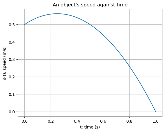
Example

Consider \(S(t)\) given by:

def S(t):
    """
    Return a value for the speed, S, as a function of time, t.
    ARGUMENTS:  t   the time
    RETURNS:    S   the speed
    """
    return 1 + 5 * t - 6 * t**2

• The following table of results is obtained:

Total distance as a function of number of steps

# intervals	increment size dt	total distance
10	0.100000	1.540000
100	0.010000	1.504900
1000	0.001000	1.500499
10000	0.000100	1.500050
100000	0.000010	1.500005

• We appear to be converging to an answer in the limit as \(\mathrm{d}t \to 0\)…

Why does this work?

• The approach above uses the fact that, at any instant in time, the speed is the rate of change in distance:

  • That is, \(\text{speed} = \dfrac{\text{change in distance}}{\text{time}}\);

  • so, \(\text{change in distance} = \text{time} \times \text{speed}\);

  • in code this can be expressed as:

    d = d + dt * s(t)
    

• We can re-arrange the last expression to get the average speed over the interval for \(t\) to \(t + \mathrm{d}t\):

  \[ S(t) = \frac{D(t+\mathrm{d}t) - D(t)}{\mathrm{d}t}. \]

• In fact, to obtain a converged answer it is necessary to take smaller and smaller choices for \(\mathrm{d}t\).

• In mathematical notation this is written as

  \[ S(t) = \lim_{\mathrm{d}t \to 0} \frac{D(t+\mathrm{d}t) - D(t)}{\mathrm{d}t}. \]

• This is what rate of change really means at each instant.

• The standard terminology for this is to say that the speed \(S(t)\) is the derivative of the distance \(d\) with respect to time \(t\).

• The notation for this is \(S(t) = D'(t)\).

A graphical interpretation

• We can give a graphical interpretation of the relationship between \(D(t)\) and its derivative \(D'(t)\).

Inspection of the plots shows that the steepness of the red curve \(D(t)\) is related to the value of the blue curve \(S(t)\):

• As the blue curve increases in value, the red curve increases in steepness.

• When the blue curve starts to decrease in value, the red curve decreases in steepness.

• By the time the blue curve has a value of zero the red curve is flat.

In fact the gradient of the red curve is precisely equal to the value of the blue curve.

This provides for an alternative interpretation of the derivative of a function…

The function \(D'(t)\) is the function whose value is equal to the slope (or gradient) of \(D(t)\) at every value of \(t\).

The derivative as a gradient

• What is the slope/gradient of a line?

• It is the steepness…

• The equation of a straight line with slope \(m\) is given by

  \[ y(t) = m t + c. \]

Slope of a curve

• What is the slope/gradient of a curve?

• The slope of the straight-line approximation (“chord”) is

  \[ \frac{y(t + \mathrm{d}t) - y(t)}{\mathrm{d}t}. \]

• We can get a better approximation by taking a smaller value for \(\mathrm{d}t\)…

• We can get an even better approximation by taking an even smaller value for \(\mathrm{d}t\)…

By taking smaller and smaller values of \(\mathrm{d}t\), it becomes clear that we can assign an instantaneous value to the slope at any point \(t\):

\[ \lim_{\mathrm{d}t \to 0} \frac{y(t+\mathrm{d}t) - y(t)}{\mathrm{d}t}. \]

But this is precisely the definition of derivative \(y'(t)\)!

Further reading

• Wikipedia: Rate of change

• Wikipedia: Speed

• Wikipedia: Derivative

• Maths is fun: Derivatives introduction

The slides used in the lecture are also available