Lecture 06: Gaussian elimination

Elementary row operations

Recall the problem is to solve a set of \(n\) linear equations for \(n\) unknown values \(x_j\), for \(j=1, 2, \ldots, n\).

Notation:

\[\begin{split} \begin{aligned} \text{Equation } 1: && a_{11} x_1 + a_{12} x_2 + a_{13} x_3 + \cdots + a_{1n} x_n & = b_1 \\ \text{Equation } 2: && a_{21} x_1 + a_{22} x_2 + a_{23} x_3 + \cdots + a_{2n} x_n & = b_2 \\ \vdots \\ \text{Equation } i: && a_{i1} x_1 + a_{i2} x_2 + a_{i3} x_3 + \cdots + a_{in} x_n & = b_i \\ \vdots \\ \text{Equation } n: && a_{n1} x_1 + a_{n2} x_2 + a_{n3} x_3 + \cdots + a_{nn} x_n & = b_n. \end{aligned} \end{split}\]

Elementary row operations

Consider equation \(p\) of the above system:

\[ a_{p1} x_1 + a_{p2} x_2 + a_{p3} x_3 + \cdots + a_{pn} x_n = b_p, \]

and equation \(q\):

\[ a_{q1} x_1 + a_{q2} x_2 + a_{q3} x_3 + \cdots + a_{qn} x_n = b_q. \]

Note three things…

• The order in which we choose to write the \(n\) equations is irrelevant

• We can multiply any equation by an arbitrary real number (\(k \neq 0\) say):

  \[ k a_{p1} x_1 + k a_{p2} x_2 + k a_{p3} x_3 + \cdots + k a_{pn} x_n = k b_p. \]

• We can add any two equations:

  \[ k a_{p1} x_1 + k a_{p2} x_2 + k a_{p3} x_3 + \cdots + k a_{pn} x_n = k b_p \]

  added to

  \[ a_{q1} x_1 + a_{q2} x_2 + a_{q3} x_3 + \cdots + a_{qn} x_n = b_q \]

  yields

  \[ (k a_{p1} + a_{q1}) x_1 + (k a_{p2} + a_{q2}) x_2 + \cdots + (k a_{pn} + a_{qn}) x_n = k b_p + b_q. \]

Example 1

Consider the system

\[\begin{split} \begin{aligned} 2 x_1 + 3 x_2 & = 4 && (1) \\ -3 x_1 + 2 x_2 & = 7 && (2). \end{aligned} \end{split}\]

• \(4 \times (1)\) \(\rightarrow\) \(8 x_1 + 12 x_2 = 16\).

• \(-1.5 \times (2)\) \(\rightarrow\) \(4.5 x_1 - 3 x_2 = -10.5\).

• \((2) + (1)\) \(\rightarrow\) \(-x_1 + 5 x_2 = 11\).

• \((2) + 1.5 \times (1)\) \(\rightarrow\) \(0 + 6.5 x_2 = 13\).

Example 2 (homework)

Consider the system

\[\begin{split} \begin{aligned} x_1 + 2 x_2 & = 1 && (3) \\ 4 x_1 + x_2 & = -3 && (4). \end{aligned} \end{split}\]

• \(2 \times (3)\) \(\rightarrow\)

• \(0.25 \times (4)\) \(\rightarrow\)

• \((4) + (-1) \times (3)\) \(\rightarrow\)

• \((4) + (-4) \times (3)\) \(\rightarrow\)

General matrix-vector form

What does this mean when we write the equations as a single matrix equation?

\[\begin{split} \begin{pmatrix} a_{11} & a_{12} & a_{13} & \cdots & a_{1n} \\ a_{21} & a_{22} & a_{23} & \cdots & a_{2n} \\ a_{31} & a_{32} & a_{33} & \cdots & a_{3n} \\ \vdots & \vdots & \vdots & & \vdots \\ a_{n1} & a_{n2} & a_{n3} & \cdots & a_{nn} \end{pmatrix} \begin{pmatrix} x_1 \\ x_2 \\ x_3 \\ \vdots \\ x_n \end{pmatrix} = \begin{pmatrix} b_1 \\ b_2 \\ b_3 \\ \vdots \\ b_n \end{pmatrix}. \end{split}\]

Recall the \(n \times n\) matrix \(A\) represents the coefficients that multiply the unknowns in each equation (row), while the \(n\)-vector \(\vec{b}\) represents the right-hand-side values.

Application to matrix equations

For a system written in matrix form our three observations mean the following:

• We can swap any two rows of the matrix (and corresponding right-hand side entries). For example:

  \[\begin{split} \begin{pmatrix} 2 & 3 \\ -3 & 2 \end{pmatrix} \begin{pmatrix} x_1 \\ x_2 \end{pmatrix} = \begin{pmatrix} 4 \\ 7 \end{pmatrix} \Rightarrow \begin{pmatrix} -3 & 2\\ 2 & 3 \end{pmatrix} \begin{pmatrix} x_1 \\ x_2 \end{pmatrix} = \begin{pmatrix} 7 \\ 4 \end{pmatrix} \end{split}\]

• We can multiply any row of the matrix (and corresponding right-hand side entry) by a scalar. For example:

  \[\begin{split} \begin{pmatrix} 2 & 3 \\ -3 & 2 \end{pmatrix} \begin{pmatrix} x_1 \\ x_2 \end{pmatrix} = \begin{pmatrix} 4 \\ 7 \end{pmatrix} \Rightarrow \begin{pmatrix} 1 & \frac{3}{2} \\ -3 & 2 \end{pmatrix} \begin{pmatrix} x_1 \\ x_2 \end{pmatrix} = \begin{pmatrix} 2 \\ 7 \end{pmatrix} \end{split}\]

• We can replace row \(q\) by row \(q + k \times\) row \(p\). For example:

  \[\begin{split} \begin{pmatrix} 2 & 3 \\ -3 & 2 \end{pmatrix} \begin{pmatrix} x_1 \\ x_2 \end{pmatrix} = \begin{pmatrix} 4 \\ 7 \end{pmatrix} \Rightarrow \begin{pmatrix} 2 & 3 \\ 0 & 6.5 \end{pmatrix} \begin{pmatrix} x_1 \\ x_2 \end{pmatrix} = \begin{pmatrix} 4 \\ 13 \end{pmatrix} \end{split}\]

  (here we replaced row \(w\) by row \(2 + 1.5 \times\) row \(1\))

  \[\begin{split} \begin{pmatrix} 1 & 2 \\ 4 & 1 \end{pmatrix} \begin{pmatrix} x_1 \\ x_2 \end{pmatrix} = \begin{pmatrix} 1 \\ -3 \end{pmatrix} \Rightarrow \begin{pmatrix} 1 & 2 \\ 0 & -7 \end{pmatrix} \begin{pmatrix} x_1 \\ x_2 \end{pmatrix} = \begin{pmatrix} 1 \\ -7 \end{pmatrix} \end{split}\]

  (here we replaced row \(2\) by row \(2 + (-4) \times\) row \(1\))

Triangular systems

Recall that we can easily solve a lower triangular system:

\[\begin{split} \begin{pmatrix} a_{11} & 0 & 0 & \cdots & 0 \\ a_{21} & a_{22} & 0 & \cdots & 0 \\ a_{31} & a_{32} & a_{33} & \cdots & 0 \\ \vdots & \vdots & \vdots & \ddots & \vdots \\ a_{n1} & a_{n2} & a_{n3} & \cdots & a_{nn} \end{pmatrix} \begin{pmatrix} x_1 \\ x_2 \\ x_3 \\ \vdots \\ x_n \end{pmatrix} = \begin{pmatrix} b_1 \\ b_2 \\ b_3 \\ \vdots \\ b_n \end{pmatrix}. \end{split}\]

• \(A\) is a lower triangular matrix if every entry above the leading diagonal is zero

  \[ a_{ij} = 0 \text{ for } j > i. \]

Similarly, we can easily solve an upper triangular system:

\[\begin{split} \begin{pmatrix} a_{11} & a_{12} & a_{13} & \cdots & a_{1n} \\ 0 & a_{22} & a_{23} & \cdots & a_{2n} \\ 0 & 0 & a_{33} & \cdots & a_{3n} \\ \vdots & \vdots & \vdots & \ddots & \vdots \\ 0 & 0 & 0 & \cdots & a_{nn} \end{pmatrix} \begin{pmatrix} x_1 \\ x_2 \\ x_3 \\ \vdots \\ x_n \end{pmatrix} = \begin{pmatrix} b_1 \\ b_2 \\ b_3 \\ \vdots \\ b_n \end{pmatrix}. \end{split}\]

• \(A\) is an upper triangular matrix if every entry below the leading diagonal is zero

  \[ a_{ij} = 0 \text{ for } i > j. \]

Strategy

• Three types of operation described above are called elementary row operations (ERO).

• We know that an upper triangular system can be easily solved… so, can we systematically apply a sequence of ERO to reduce an arbitrary system to triangular form?

• The answer is “yes”… and the algorithm for doing this is known as forward elimination or (more commonly) as Gaussian elimination (GE).

Gaussian elimination

First appeared in China…

From Wikipedia:

The method of Gaussian elimination appears in the Chinese mathematical text Chapter Eight: Rectangular Arrays of The Nine Chapters on the Mathematical Art. Its use is illustrated in eighteen problems, with two to five equations. The first reference to the book by this title is dated to 179 CE, but parts of it were written as early as approximately 150 BCE. It was commented on by Liu Hui in the 3rd century.

The method in Europe stems from the notes of Isaac Newton. In 1670, he wrote that all the algebra books known to him lacked a lesson for solving simultaneous equations, which Newton then supplied. Carl Friedrich Gauss in 1810 devised a notation for symmetric elimination that was adopted in the 19th century by professional hand computers to solve the normal equations of least-squares problems. The algorithm that is taught in high school was named for Gauss only in the 1950s as a result of confusion over the history of the subject.

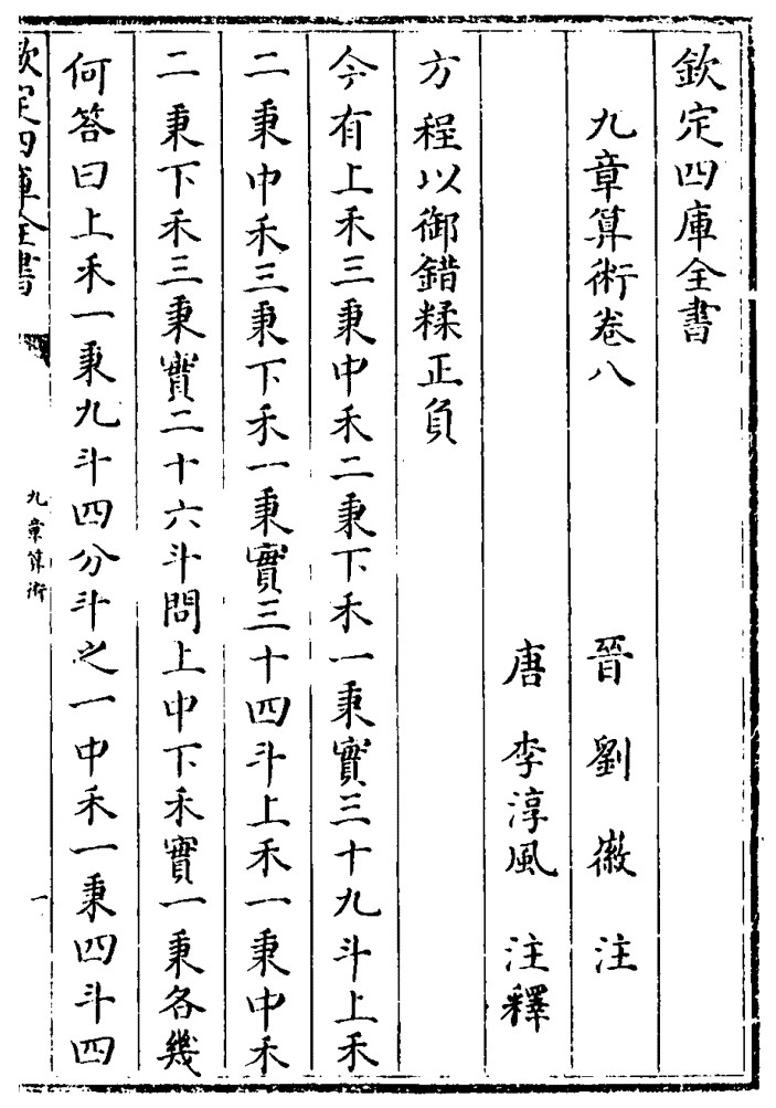
Fig. 3 Image from Nine Chapter of the Mathematical art

The algorithm

The following algorithm systematically introduces zeros into the system of equations, below the diagonal.

1. Subtract multiples of row 1 from the rows below it to eliminate (make zero) nonzero entries in column 1.

2. Subtract multiplies of the new row 2 from the rows below it to eliminate nonzero entries in column 2.

3. Repeat for row \(3, 4, \ldots, n-1\).

After row \(n-1\) all entities below the diagonal have been eliminated, so \(A\) is now upper triangular and the resulting system can be solved by backward substitution.

Example 1

Use Gaussian eliminate to solve the linear system of equations given by

\[\begin{split} \begin{pmatrix} 2 & 1 & 4 \\ 1 & 2 & 2 \\ 2 & 4 & 6 \end{pmatrix} \begin{pmatrix} x_1 \\ x_2 \\ x_3 \end{pmatrix} = \begin{pmatrix} 12 \\ 9 \\ 22 \end{pmatrix}. \end{split}\]

First, use the first row to eliminate the first column below the diagonal:

• (row 2) \(- 0.5 \times\) (row 1) gives

  \[\begin{split} \begin{pmatrix} 2 & 1 & 4 \\ \mathbf{0} & 1.5 & 0 \\ 2 & 4 & 6 \end{pmatrix} \begin{pmatrix} x_1 \\ x_2 \\ x_3 \end{pmatrix} = \begin{pmatrix} 12 \\ 3 \\ 22 \end{pmatrix} \end{split}\]

• (row 3) \(-\) (row 1) then gives

  \[\begin{split} \begin{pmatrix} 2 & 1 & 4 \\ \mathbf{0} & 1.5 & 0 \\ \mathbf{0} & 3 & 2 \end{pmatrix} \begin{pmatrix} x_1 \\ x_2 \\ x_3 \end{pmatrix} = \begin{pmatrix} 12 \\ 3 \\ 10 \end{pmatrix} \end{split}\]

Now use the second row to eliminate the second column below the diagonal.

• (row 3) \(- 2 \times\) (row 2) gives

  \[\begin{split} \begin{pmatrix} 2 & 1 & 4 \\ \mathbf{0} & 1.5 & 0 \\ \mathbf{0} & \mathbf{0} & 2 \end{pmatrix} \begin{pmatrix} x_1 \\ x_2 \\ x_3 \end{pmatrix} = \begin{pmatrix} 12 \\ 3 \\ 4 \end{pmatrix} \end{split}\]

The system is now in upper triangular form and can be solved using backward substitution to give \(\vec{x} = (1, 2, 2)^T\) (see the final example from previous lecture).

Example 2 (homework)

Use Gaussian elimination to solve the linear system of equations given by

\[\begin{split} \begin{pmatrix} 4 & -1 & -1 \\ 2 & 4 & 2 \\ 1 & 2 & 4 \end{pmatrix} \begin{pmatrix} x_1 \\ x_2 \\ x_3 \end{pmatrix} = \begin{pmatrix} 9 \\ -6 \\ 3 \end{pmatrix}. \end{split}\]

Notes

• Each row \(i\) is used to eliminate the entries in column \(i\) below \(a_{ii}\), i.e. it forces \(a_{ji} = 0\) for \(j > i\).

• This is done by subtracting a multiple of row \(i\) from row \(j\):

  \[ (\text{row } j) \leftarrow (\text{row } j) - \frac{a_{ji}}{a_{ii}} (\text{row } i). \]

• This guarantees that \(a_{ji}\) becomes zero because

  \[ a_{ji} \leftarrow a_{ji} - \frac{a_{ji}}{a_{ii}} a_{ii} = a_{ji} - a_{ji} = 0. \]

Example 3 (homework)

Solve the system

\[\begin{split} \begin{pmatrix} 4 & 3 & 2 & 1 \\ 1 & 2 & 2 & 2 \\ 1 & 1 & 3 & 0 \\ 2 & 1 & 2 & 3 \end{pmatrix} \begin{pmatrix} x_1 \\ x_2 \\ x_3 \\ x_4 \end{pmatrix} = \begin{pmatrix} 10 \\ 7 \\ 5 \\ 8 \end{pmatrix}. \end{split}\]

The solution is \(\vec{x} = (1, 1, 1, 1)^T\).

Final Notes

GE can be used to solve linear systems of equations…

• The computational cost is \(O(n^3)\) – which can be quite high for large values of \(n\).

• Problems can occur if \(\,a_{ii} = 0\,\) for any \(i\) in a row that is being used to do the elimination;

• Can overcome by swapping row \(i\) with any row beneath (more later).

• If \(\,a_{ii} = 0\,\) for a row that is being used to do the elimination, and all rows beneath have a zero in column \(i\), then the GE algorithm breaks down.

• The GE algorithm will only break down if the system is singular (so no solution exists or no unique solution).

• If the unique solution does exist the GE algorithm (with row swapping if needed) will find it!

Further reading

• Wikipedia: Gaussian elimination

• Joseph F. Grcar. How ordinary elimination became Gaussian elimination. Historia Mathematica. Volume 38, Issue 2, May 2011. (More history)

• The method is usually implemented via the LU factorisation method we learn next!