Lecture 12: Derivatives and differential equations#
Recap#
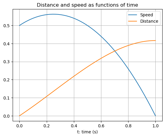
We discussed the concept of rate of change
speed is the rate of change of distance;
instantaneous speed is the limit of average speeds over shorter and shorter time periods,
\[ \frac{D(t + \mathrm{d}t) - D(t)}{\mathrm{d}t} \text{ as } \mathrm{d}t \to 0; \]instantaneous rate of change as the limit of
\[ \frac{(\text{value at time } t + \mathrm{d}t) - (\text{value at time } t)}{\mathrm{d}t} \text{ as } \mathrm{d}t \to 0. \]
We defined the derivative of a function \(y(t)\) by
\[ y'(t) = \lim_{\mathrm{d}t \to 0} \frac{y(t+\mathrm{d}t) - y(t)}{\mathrm{d}t}. \]We saw that speed, \(S(t)\), is the derivative of distance covered, \(D(t)\):
\[ S(t) = D'(t) = \lim_{\mathrm{d}t \to 0} \frac{D(t+\mathrm{d}t) - D(t)}{\mathrm{d}t}. \]We saw a geometric interpretation of the derivative of \(y(t)\) by considering the slope of its graph:
The slope of the straight line approximation (chord) is
\[ \frac{y(t + \mathrm{d}t) - y(t)}{\mathrm{d}t}. \]
Graphs and derivatives#
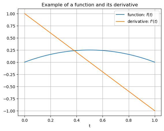
We now know a geometric interpretation of the derivative of a function, as being equal to the function’s slope at each point.
This means we can sketch an approximation to the derivative of any given function.
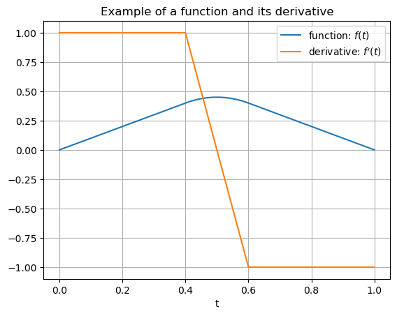
In the following examples, the graph of a function \(y(t)\) is given and the graph of \(y'(t)\) is then approximated.
Example 1#
Example 2#
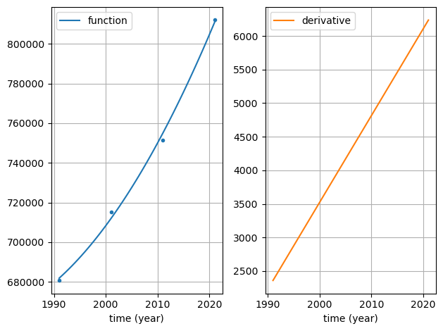
Example 3#
The population of Leeds over time (fitted):
Differential equations#
We have already seen that, for speed, \(S(t) = D'(t)\).
What is the rate of change of speed?
Answer: acceleration, \(a(t)\) say:
a positive value for \(a(t)\) means that speed is increasing whilst a negative value means that speed is decreasing.
When a model takes the form of an equation which involves one or more derivatives then it is called a differential equation.
We have already seen (and computationally solved) a simple example of a differential equation:
\[ D'(t) = 1 + 5t - 6t^2 \]where \(D(0) = 0\).
Most models of dynamic processes take the form of differential equations.
The following example uses the fact that the acceleration of an object is equal to the rate of change of its speed:
i.e. \(a(t) = S'(t)\).
An object in free fall#
Consider a simple model for an object falling from a large height, based on the two following assumptions:
all objects are attracted downward with an acceleration due to gravity of \(9.81 \, \mathrm{m} / \mathrm{s}^2\);
air resistance causes an object to decelerate in proportion to its speed (i.e., the faster it travels the greater the air resistance).
What is the net acceleration on the object?
If it is falling with speed \(S(t)\) the net acceleration downwards is \(g - kS(t)\) for some constant \(k\).
This results in the following differential equation:
\[ S'(t) = g - k S(t). \]How could we solve this equation?
Recall how we solved \(D'(t) = 1 + 5t - 6t^2\)?
We can do a similar thing again: divide the time period into lots of small intervals and assume everything is approximately constant on each time interval.
We know that
\[ S'(t) = \lim_{\mathrm{d}t \to 0} \frac{S(t + \mathrm{d}t) - S(t)}{\mathrm{d}t} \approx \frac{S(t+ \mathrm{d}t) - S(t)}{\mathrm{d}t} \]for a small value of \(\mathrm{d}t\).
Hence we can say that:
\[ S(t + \mathrm{d}t) = S(t) + \mathrm{d}t (g - k S(t)). \]
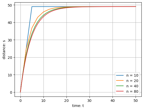
Python algorithm:#
def freefall(n):
    """
    Plot the trajectory of an object falling freely.
    Input: n number of timesteps
    """

    tfinal = 50.0  # Select the final time
    g = 9.81  # acceleration due to gravity (m/s)
    k = 0.2  # air resistance coefficient

    # initialise time and speed arrays array
    t = np.zeros([n + 1, 1])
    s = np.zeros([n + 1, 1])

    # set initial conditions
    s[0] = 0.0
    t[0] = 0.0

    dt = (tfinal - t[0]) / n  # calculate step size

    # take n time steps, in which it is assumed that the acceleration
    # is constant in each small time interval
    for i in range(n):
        t[i + 1] = t[i] + dt
        s[i + 1] = s[i] + dt * (g - k * s[i])

    # plot output
    plt.plot(t, s, label=f"n = {n}")
Python algorithm: Results#
Euler’s method#
The approach we have used applies for any differential equation involving just a single derivative.
It is called Euler’s method.
We can always arrange such an equation in the form:
\[ y'(t) = f(t, y) \quad \text{ subject to the initial condition } \quad y(t_0) = y_0. \]Examples:
\(y'(t) = 1+ 5t - 6t^2\) and \(y(0) = 0\).
\(y'(t) = g- ky\) and \(y(0) =0\).
\(y'(t) = -y^2 + \frac{1}{t}\) and \(y(1) = 2\).
For the general equation we have the following algorithm:
Set initial values \(t^{(0)}\) and \(y^{(0)}\).
Loop over all time steps, until the final time, updating using the formulae:
\[\begin{split} \begin{aligned} y^{(i+1)} & = y^{(i)} + \mathrm{d}t f(t^{(i)}, y^{(i)}) \\ t^{(i+1)} & = t^{(i)} + \mathrm{d}t. \end{aligned} \end{split}\]
Example#
Take three steps of Euler’s method to approximate the solution of
\[ y'(t) = -y^2 + \frac{1}{t} \text{ subject to the initial condition } y(1) = 2 \]for \(1 \le t \le 2\).
For this example we have:
\(n = 3\)
\(t_0 = 1\)
\(y_0 = 2\)
\(t_{\text{final}} = 2\)
\(\mathrm{d}t = (2-1)/3 = 1/3\)
\(f(t, y) = -y^2 + 1/t\).
Summary#
Given the graph of \(y(t)\) it is possible to sketch the graph of \(y'(t)\) (with some care!).
Computational models which involve dynamic processes usually involve the use of derivatives.
An equation which includes a derivative is known as a differential equation.
To solve a differential equation it is necessary to know some information about the solution at some starting point (e.g. initial distance travelled, initial speed, population at a given point in time, etc.).
One computational approach to solve such equations is Euler’s method - which gets more accurate with more sub-intervals used.
Further reading#
Wikipedia: Differential equations
Maths is fun: Differential equations
Wikipedia: Euler method
x-engineer: Euler integration method for solving differential equations
Euler’s method in films:
Catherine Meyers, Exploring the Math in `Hidden Figures’, Inside Science, 2017.
The slides used in the lecture are also available