WS01: Introduction to Python and Jupyter

WS01: Introduction to Python and Jupyter#

This workbook is for you to get to grips with how the rest of the worksheets in this class will work and gain familiarity with Python and jupyter. You should read the text and follow the instructions of how to run each cell.

If you are familiar with the content you may go quickly through this tutorial.

What is Python?#

Python is an easy to learn, powerful programming language. It has efficient high-level data structures and a simple but effective approach to object-oriented programming. Python’s elegant syntax and dynamic typing, together with its interpreted nature, make it an ideal language for scripting and rapid application development in many areas on most platforms.

The Python interpreter and the extensive standard library are freely available in source or binary form for all major platforms from the Python web site, https://www.python.org/, and may be freely distributed. The same site also contains distributions of and pointers to many free third party Python modules, programs and tools, and additional documentation.

More: https://docs.python.org/3/tutorial

Accessing Python#

There’s a good chance that you already have Python on your operating system.

If so, you do not need to install or configure anything else to use Python. Having said that, I would strongly recommend that you install the tools and libraries described in the guides below before you start building Python applications for use in this course.

More: https://docs.python-guide.org/starting/installation/

Using Python on a School of Computing machine#

On a School of Computing machine you can access an upto date version of python using anaconda:

$ module load legacy-eng
$ module add anaconda3/2020.11

You test your version of Python by running:

$ python --version
Python 3.8.5

Using python on your own device#

You are recommended to install Anaconda and python 3. Anaconda is gives up to date version of python and python libraries which you can use during this module.

Choosing this option will require an initial software installation and routine updates. For this course the recommended package is Anaconda available from Continuum Analytics. Downloading and installing the software is well documented and easy to follow. Allow about 10-30 minutes for the installation depending on your connection speed.

You will require the following python libraries:

numpy
matplotlib
scipy (optional)

These can be installed by calling

$ conda install numpy matplotlib scipy

There is no requirement to submit code that works on a School of Computing machine for this module.

What is Jupyter?#

Jupyter notebooks are documents that can be viewed and executed inside any modern web browser. Since you’re reader this notebook, you already know how to view a Jupyter Notebook. The next step is to learn how to execute comptuations that may be embedded in a Jupyter Notebook.

To execute Python code in a notebook you will need access to a Python kernal. A kernal is simply a program that runs in the background, maintains workspace memory for variables and functions, and executes Python code. The kernal can be located on the same laptop as your web browser or located in an on-line cloud service.

We recommend the use of jupyter lab which is the next generation web-based interface for jupyter notebooks.

See this video for a brief introduction:

from IPython.display import YouTubeVideo

YouTubeVideo("A5YyoCKxEOU", 560, 315, rel=0)

Using Jupyter on a School of Computing machine#

If you have followed the same module add anaconda3/2020.11 etc instructions from before to load Python, you will already have Jupyter Lab installed.

Using Jupyter in the cloud#

The easiest way to use Jupyter notebooks is to sign up for a free or paid account on a cloud-based service such as binder, Google Colab or Deep note. Note that the free services are generally heavily oversubscribed, so you should consider a paid account to assure access during prime hours.

We have already created the links on binder for you to use. Simply click to . Each notebook in this course will have a similar logo at the top so that you can launch that notebook in binder too.

Using Jupyter on your own laptop#

For regular off-line use you should consider installing a Jupyter Notebook/Python environment directly on your laptop. This will provide you with reliable off-line access to a computational environment. This will also allow you to install additional code libraries to meet particular needs.

To install jupyterlab you should write:

$ conda install -c conda-forge jupyterlab

Step 1: Start a jupyter notebook session#

If you are using a cloud-based service a Jupyter session will be started when you log on.

If you have installed Jupyter on your own laptop or on a School of Computing machine you can open a Jupyter session from a terminal:

$ jupyter lab

Either way, once you have opened the session you should see a browser window like this:

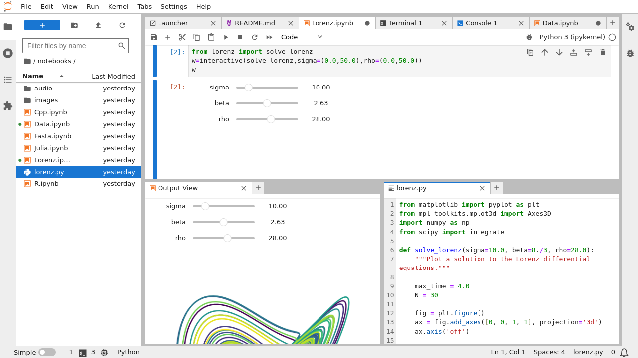
If you are unfamiliar with jupyter lab or jupyter notebooks we recommend you follow the user documentation. Alternatively we give a brief guide below.

Running cells#

A notebook’s cells default to code whenever you first create one, and that cell uses the kernal that you chose when you started your notebook.

To verify everything is working, you can add some python code to the cells and try running its contents.

print("Hello jupyter")
a = 3
b = 2
print(a + b)

Running a cell means that you will execute the cell’s contents. To execute a cell, you can just select the cell and click Run button that is in the row of buttons along the top. It’s towards the middle. If you prefer using your keyboard, you can just press “Shift” and “Enter”.

If you have multiple cells in your Notebook, and you run the cells in order, you can share your variables and imports across cells. This makes it easy to separate out your code into logical chunks without needing to reimport libraries or recreate variables or functions in every cell.

When you run a cell, you will notice that there are some square braces next to the word In to the left of the cell. The square braces will auto fill with a number that indicates the order that you ran the cells. For example, if you open a fresh Notebook and run the first cell at the top of the Notebook, the square braces will fill with the number 1.

Since the kernel is always running you code that you have executed just builds up on top of previous code. When submitted coursework or worksheet solutions you should always "Restart kernel and rerun" before submitting your work!!

Step 2: Simple calculations with python#

Python is an elegant and modern language for programming and problem solving that has found increasing use by engineers and scientists. In the next few cells we’ll demonstrate some basic functionality.

We take the following from https://learnxinyminutes.com/docs/python/. If you are already familiar with python you may wish to skip this section.

# Single line comments start with a number symbol.

""" Multiline strings can be written
    using three "s, and are often used
    as documentation.
"""

### Primitive Data types and Operators

# You have numbers
3  # => 3

# Math is what you would expect
+ 1  # => 2
- 1  # => 7
* 2  # => 20
/ 5  # => 7.0

# Integer division rounds down for both positive and negative numbers.
5 // 3  # => 1
-5 // 3  # => -2
5.0 // 3.0  # => 1.0 # works on floats too
-5.0 // 3.0  # => -2.0

# The result of division is always a float
10.0 / 3  # => 3.3333333333333335

# Modulo operation
7 % 3  # => 1
# i % j have the same sign as j, unlike C
-7 % 3  # => 2

# Exponentiation (x**y, x to the yth power)
2**3  # => 8

# Enforce precedence with parentheses
1 + 3 * 2  # => 7
(1 + 3) * 2  # => 8

# Boolean values are primitives (Note: the capitalization)
True  # => True
False  # => False

# negate with not
not True  # => False
not False  # => True

# Boolean Operators
# Note "and" and "or" are case-sensitive
True and False  # => False
False or True  # => True

# True and False are actually 1 and 0 but with different keywords
True + True  # => 2
True * 8  # => 8
False - 5  # => -5

# Comparison operators look at the numerical value of True and False
0 == False  # => True
1 == True  # => True
2 == True  # => False
-5 != False  # => True

# Using boolean logical operators on ints casts them to booleans for evaluation, but their non-cast value is returned
# Don't mix up with bool(ints) and bitwise and/or (&,|)
bool(0)  # => False
bool(4)  # => True
bool(-6)  # => True
0 and 2  # => 0
-5 or 0  # => -5

# Equality is ==
1 == 1  # => True
2 == 1  # => False

# Inequality is !=
1 != 1  # => False
2 != 1  # => True

# More comparisons
< 10  # => True
> 10  # => False
<= 2  # => True
>= 2  # => True

# Seeing whether a value is in a range
1 < 2 and 2 < 3  # => True
2 < 3 and 3 < 2  # => False
# Chaining makes this look nicer
1 < 2 < 3  # => True
2 < 3 < 2  # => False

# (is vs. ==) is checks if two variables refer to the same object, but == checks
# if the objects pointed to have the same values.
a = [1, 2, 3, 4]  # Point a at a new list, [1, 2, 3, 4]
b = a  # Point b at what a is pointing to
b is a  # => True, a and b refer to the same object
b == a  # => True, a's and b's objects are equal
b = [1, 2, 3, 4]  # Point b at a new list, [1, 2, 3, 4]
b is a  # => False, a and b do not refer to the same object
b == a  # => True, a's and b's objects are equal

# Strings are created with " or '
"This is a string."
"This is also a string."

# Strings can be added too
"Hello " + "world!"  # => "Hello world!"
# String literals (but not variables) can be concatenated without using '+'
"Hello " "world!"  # => "Hello world!"

# A string can be treated like a list of characters
"Hello world!"[0]  # => 'H'

# You can find the length of a string
len("This is a string")  # => 16

# You can also format using f-strings or formatted string literals (in Python 3.6+)
name = "Reiko"
f"She said her name is {name}."  # => "She said her name is Reiko"
# You can basically put any Python expression inside the braces and it will be output in the string.
f"{name} is {len(name)} characters long."  # => "Reiko is 5 characters long."

# None is an object
None  # => None

# Don't use the equality "==" symbol to compare objects to None
# Use "is" instead. This checks for equality of object identity.
"etc" is None  # => False <-- this gives a warning since "etc" is clearly not None!!
None is None  # => True

# None, 0, and empty strings/lists/dicts/tuples/sets all evaluate to False.
# All other values are True
bool(0)  # => False
bool("")  # => False
bool([])  # => False
bool({})  # => False
bool(())  # => False
bool(set())  # => False

Variables and collections#

# Python has a print function
print("I'm Python. Nice to meet you!")  # => I'm Python. Nice to meet you!

# By default the print function also prints out a newline at the end.
# Use the optional argument end to change the end string.
print("Hello, World", end="!")  # => Hello, World!

# Simple way to get input data from console
input_string_var = input("Enter some data: ")  # Returns the data as a string

# There are no declarations, only assignments.
# Convention is to use lower_case_with_underscores
some_var = 5
some_var  # => 5

# Accessing a previously unassigned variable is an exception.
# See Control Flow to learn more about exception handling.
some_unknown_var  # Raises a NameError

# if can be used as an expression
# Equivalent of C's '?:' ternary operator
"yay!" if 0 > 1 else "nay!"  # => "nay!"

# Lists store sequences
li = []
# You can start with a prefilled list
other_li = [4, 5, 6]

# Add stuff to the end of a list with append
li.append(1)  # li is now [1]
li.append(2)  # li is now [1, 2]
li.append(4)  # li is now [1, 2, 4]
li.append(3)  # li is now [1, 2, 4, 3]
# Remove from the end with pop
li.pop()  # => 3 and li is now [1, 2, 4]
# Let's put it back
li.append(3)  # li is now [1, 2, 4, 3] again.

# Access a list like you would any array
li[0]  # => 1
# Look at the last element
li[-1]  # => 3

# Looking out of bounds is an IndexError
li[4]  # Raises an IndexError

# You can look at ranges with slice syntax.
# The start index is included, the end index is not
# (It's a closed/open range for you mathy types.)
li[1:3]  # Return list from index 1 to 3 => [2, 4]
li[2:]  # Return list starting from index 2 => [4, 3]
li[:3]  # Return list from beginning until index 3  => [1, 2, 4]
li[::2]  # Return list selecting every second entry => [1, 4]
li[::-1]  # Return list in reverse order => [3, 4, 2, 1]
# Use any combination of these to make advanced slices
# li[start:end:step]

# Make a one layer deep copy using slices
li2 = li[:]  # => li2 = [1, 2, 4, 3] but (li2 is li) will result in false.

# Remove arbitrary elements from a list with "del"
del li[2]  # li is now [1, 2, 3]

# Remove first occurrence of a value
li.remove(2)  # li is now [1, 3]
li.remove(2)  # Raises a ValueError as 2 is not in the list

# Insert an element at a specific index
li.insert(1, 2)  # li is now [1, 2, 3] again

# Get the index of the first item found matching the argument
li.index(2)  # => 1
li.index(4)  # Raises a ValueError as 4 is not in the list

# You can add lists
# Note: values for li and for other_li are not modified.
li + other_li  # => [1, 2, 3, 4, 5, 6]

# Concatenate lists with "extend()"
li.extend(other_li)  # Now li is [1, 2, 3, 4, 5, 6]
li

# Check for existence in a list with "in"
1 in li  # => True

# Examine the length with "len()"
len(li)  # => 6

# Tuples are like lists but are immutable.
tup = (1, 2, 3)
tup[0]  # => 1
tup[0] = 3  # Raises a TypeError

# Note that a tuple of length one has to have a comma after the last element but
# tuples of other lengths, even zero, do not.
type((1))  # => <class 'int'>
type((1,))  # => <class 'tuple'>
type(())  # => <class 'tuple'>

# You can do most of the list operations on tuples too
len(tup)  # => 3
tup + (4, 5, 6)  # => (1, 2, 3, 4, 5, 6)
tup[:2]  # => (1, 2)
2 in tup  # => True

# You can unpack tuples (or lists) into variables
a, b, c = (1, 2, 3)  # a is now 1, b is now 2 and c is now 3
# You can also do extended unpacking
a, *b, c = (1, 2, 3, 4)  # a is now 1, b is now [2, 3] and c is now 4
# Tuples are created by default if you leave out the parentheses
d, e, f = 4, 5, 6  # tuple 4, 5, 6 is unpacked into variables d, e and f
# respectively such that d = 4, e = 5 and f = 6
# Now look how easy it is to swap two values
e, d = d, e  # d is now 5 and e is now 4

# Dictionaries store mappings from keys to values
empty_dict = {}
# Here is a prefilled dictionary
filled_dict = {"one": 1, "two": 2, "three": 3}

# Note keys for dictionaries have to be immutable types. This is to ensure that
# the key can be converted to a constant hash value for quick look-ups.
# Immutable types include ints, floats, strings, tuples.
invalid_dict = {[1, 2, 3]: "123"}  # => Raises a TypeError: unhashable type: 'list'
valid_dict = {(1, 2, 3): [1, 2, 3]}  # Values can be of any type, however.

# Look up values with []
filled_dict["one"]  # => 1

# Get all keys as an iterable with "keys()". We need to wrap the call in list()
# to turn it into a list. We'll talk about those later.  Note - for Python
# versions <3.7, dictionary key ordering is not guaranteed. Your results might
# not match the example below exactly. However, as of Python 3.7, dictionary
# items maintain the order at which they are inserted into the dictionary.
list(filled_dict.keys())  # => ["three", "two", "one"] in Python <3.7
list(filled_dict.keys())  # => ["one", "two", "three"] in Python 3.7+

# Get all values as an iterable with "values()". Once again we need to wrap it
# in list() to get it out of the iterable. Note - Same as above regarding key
# ordering.
list(filled_dict.values())  # => [3, 2, 1]  in Python <3.7
list(filled_dict.values())  # => [1, 2, 3] in Python 3.7+

# Check for existence of keys in a dictionary with "in"
"one" in filled_dict  # => True
1 in filled_dict  # => False

# Looking up a non-existing key is a KeyError
filled_dict["four"]  # KeyError

# Use "get()" method to avoid the KeyError
filled_dict.get("one")  # => 1
filled_dict.get("four")  # => None
# The get method supports a default argument when the value is missing
filled_dict.get("one", 4)  # => 1
filled_dict.get("four", 4)  # => 4

# "setdefault()" inserts into a dictionary only if the given key isn't present
filled_dict.setdefault("five", 5)  # filled_dict["five"] is set to 5
filled_dict.setdefault("five", 6)  # filled_dict["five"] is still 5

# Adding to a dictionary
filled_dict.update({"four": 4})  # => {"one": 1, "two": 2, "three": 3, "four": 4}
filled_dict["four"] = 4  # another way to add to dict

# Remove keys from a dictionary with del
del filled_dict["one"]  # Removes the key "one" from filled dict

# From Python 3.5 you can also use the additional unpacking options
{"a": 1, **{"b": 2}}  # => {'a': 1, 'b': 2}
{"a": 1, **{"a": 2}}  # => {'a': 2}

# Sets store ... well sets
empty_set = set()
# Initialize a set with a bunch of values. Yeah, it looks a bit like a dict. Sorry.
some_set = {1, 1, 2, 2, 3, 4}  # some_set is now {1, 2, 3, 4}

# Similar to keys of a dictionary, elements of a set have to be immutable.
invalid_set = {[1], 1}  # => Raises a TypeError: unhashable type: 'list'
valid_set = {(1,), 1}

# Add one more item to the set
filled_set = some_set
filled_set.add(5)  # filled_set is now {1, 2, 3, 4, 5}
# Sets do not have duplicate elements
filled_set.add(5)  # it remains as before {1, 2, 3, 4, 5}

# Do set intersection with &
other_set = {3, 4, 5, 6}
filled_set & other_set  # => {3, 4, 5}

# Do set union with |
filled_set | other_set  # => {1, 2, 3, 4, 5, 6}

# Do set difference with -
{1, 2, 3, 4} - {2, 3, 5}  # => {1, 4}

# Do set symmetric difference with ^
{1, 2, 3, 4} ^ {2, 3, 5}  # => {1, 4, 5}

# Check if set on the left is a superset of set on the right
{1, 2} >= {1, 2, 3}  # => False

# Check if set on the left is a subset of set on the right
{1, 2} <= {1, 2, 3}  # => True

# Check for existence in a set with in
2 in filled_set  # => True
10 in filled_set  # => False

# Make a one layer deep copy
filled_set = some_set.copy()  # filled_set is {1, 2, 3, 4, 5}
filled_set is some_set  # => False

Control flow and iterables#

# Let's just make a variable
some_var = 5

# Here is an if statement. Indentation is significant in Python!
# Convention is to use four spaces, not tabs.
# This prints "some_var is smaller than 10"
if some_var > 10:
    print("some_var is totally bigger than 10.")
elif some_var < 10:  # This elif clause is optional.
    print("some_var is smaller than 10.")
else:  # This is optional too.
    print("some_var is indeed 10.")

"""
For loops iterate over lists
prints:
    dog is a mammal
    cat is a mammal
    mouse is a mammal
"""
for animal in ["dog", "cat", "mouse"]:
    # You can use format() to interpolate formatted strings
    print("{} is a mammal".format(animal))

"""
"range(number)" returns an iterable of numbers
from zero to the given number
prints:
    0
    1
    2
    3
"""
for i in range(4):
    print(i)

"""
"range(lower, upper)" returns an iterable of numbers
from the lower number to the upper number
prints:
    4
    5
    6
    7
"""
for i in range(4, 8):
    print(i)

"""
"range(lower, upper, step)" returns an iterable of numbers
from the lower number to the upper number, while incrementing
by step. If step is not indicated, the default value is 1.
prints:
    4
    6
"""
for i in range(4, 8, 2):
    print(i)

"""
To loop over a list, and retrieve both the index and the value of each item in the list
prints:
    0 dog
    1 cat
    2 mouse
"""
animals = ["dog", "cat", "mouse"]
for i, value in enumerate(animals):
    print(i, value)

"""
While loops go until a condition is no longer met.
prints:
    0
    1
    2
    3
"""
x = 0
while x < 4:
    print(x)
    x += 1  # Shorthand for x = x + 1

# Handle exceptions with a try/except block
try:
    # Use "raise" to raise an error
    raise IndexError("This is an index error")
except IndexError as e:
    pass  # Pass is just a no-op. Usually you would do recovery here.
except (TypeError, NameError):
    pass  # Multiple exceptions can be handled together, if required.
else:  # Optional clause to the try/except block. Must follow all except blocks
    print("All good!")  # Runs only if the code in try raises no exceptions
finally:  # Execute under all circumstances
    print("We can clean up resources here")

# Instead of try/finally to cleanup resources you can use a with statement
with open("myfile.txt") as f:
    for line in f:
        print(line)

# Writing to a file
contents = {"aa": 12, "bb": 21}
with open("myfile1.txt", "w+") as file:
    file.write(str(contents))  # writes a string to a file

import json

with open("myfile2.txt", "w+") as file:
    file.write(json.dumps(contents))  # writes an object to a file

# Reading from a file
with open("myfile1.txt", "r+") as file:
    contents = file.read()  # reads a string from a file
print(contents)
# print: {"aa": 12, "bb": 21}

with open("myfile2.txt", "r+") as file:
    contents = json.load(file)  # reads a json object from a file
print(contents)
# print: {"aa": 12, "bb": 21}

# Python offers a fundamental abstraction called the Iterable.
# An iterable is an object that can be treated as a sequence.
# The object returned by the range function, is an iterable.

filled_dict = {"one": 1, "two": 2, "three": 3}
our_iterable = filled_dict.keys()
print(
    our_iterable
)  # => dict_keys(['one', 'two', 'three']). This is an object that implements our Iterable interface.

# We can loop over it.
for i in our_iterable:
    print(i)  # Prints one, two, three

# However we cannot address elements by index.
our_iterable[1]  # Raises a TypeError

# An iterable is an object that knows how to create an iterator.
our_iterator = iter(our_iterable)

# Our iterator is an object that can remember the state as we traverse through it.
# We get the next object with "next()".
next(our_iterator)  # => "one"

# It maintains state as we iterate.
next(our_iterator)  # => "two"
next(our_iterator)  # => "three"

# After the iterator has returned all of its data, it raises a StopIteration exception
next(our_iterator)  # Raises StopIteration

# We can also loop over it, in fact, "for" does this implicitly!
our_iterator = iter(our_iterable)
for i in our_iterator:
    print(i)  # Prints one, two, three

# You can grab all the elements of an iterable or iterator by calling list() on it.
list(our_iterable)  # => Returns ["one", "two", "three"]
list(our_iterator)  # => Returns [] because state is saved

Function#

# Use "def" to create new functions
def add(x, y):
    print("x is {} and y is {}".format(x, y))
    return x + y  # Return values with a return statement

# Calling functions with parameters
add(5, 6)  # => prints out "x is 5 and y is 6" and returns 11

# Another way to call functions is with keyword arguments
add(y=6, x=5)  # Keyword arguments can arrive in any order.

# You can define functions that take a variable number of
# positional arguments
def varargs(*args):
    return args


varargs(1, 2, 3)  # => (1, 2, 3)

# You can define functions that take a variable number of
# keyword arguments, as well
def keyword_args(**kwargs):
    return kwargs


# Let's call it to see what happens
keyword_args(big="foot", loch="ness")  # => {"big": "foot", "loch": "ness"}

# You can do both at once, if you like
def all_the_args(*args, **kwargs):
    print(args)
    print(kwargs)


"""
all_the_args(1, 2, a=3, b=4) prints:
    (1, 2)
    {"a": 3, "b": 4}
"""

# When calling functions, you can do the opposite of args/kwargs!
# Use * to expand tuples and use ** to expand kwargs.
args = (1, 2, 3, 4)
kwargs = {"a": 3, "b": 4}
all_the_args(*args)  # equivalent to all_the_args(1, 2, 3, 4)
all_the_args(**kwargs)  # equivalent to all_the_args(a=3, b=4)
all_the_args(*args, **kwargs)  # equivalent to all_the_args(1, 2, 3, 4, a=3, b=4)

# Returning multiple values (with tuple assignments)
def swap(x, y):
    return y, x  # Return multiple values as a tuple without the parenthesis.
    # (Note: parenthesis have been excluded but can be included)


x = 1
y = 2
x, y = swap(x, y)  # => x = 2, y = 1
# (x, y) = swap(x,y)  # Again parenthesis have been excluded but can be included.

# Function Scope
x = 5


def set_x(num):
    # Local var x not the same as global variable x
    x = num  # => 43
    print(x)  # => 43


def set_global_x(num):
    global x
    print(x)  # => 5
    x = num  # global var x is now set to 6
    print(x)  # => 6


set_x(43)
set_global_x(6)

# Python has first class functions
def create_adder(x):
    def adder(y):
        return x + y

    return adder


add_10 = create_adder(10)
add_10(3)  # => 13

# There are also anonymous functions
(lambda x: x > 2)(3)  # => True
(lambda x, y: x**2 + y**2)(2, 1)  # => 5

# There are built-in higher order functions
list(map(add_10, [1, 2, 3]))  # => [11, 12, 13]
list(map(max, [1, 2, 3], [4, 2, 1]))  # => [4, 2, 3]

list(filter(lambda x: x > 5, [3, 4, 5, 6, 7]))  # => [6, 7]

# We can use list comprehensions for nice maps and filters
# List comprehension stores the output as a list which can itself be a nested list
[add_10(i) for i in [1, 2, 3]]  # => [11, 12, 13]
[x for x in [3, 4, 5, 6, 7] if x > 5]  # => [6, 7]

# You can construct set and dict comprehensions as well.
{x for x in "abcddeef" if x not in "abc"}  # => {'d', 'e', 'f'}
{x: x**2 for x in range(5)}  # => {0: 0, 1: 1, 2: 4, 3: 9, 4: 16}

Modules#

# You can import modules
import math

print(math.sqrt(16))  # => 4.0

# You can get specific functions from a module
from math import ceil, floor

print(ceil(3.7))  # => 4.0
print(floor(3.7))  # => 3.0

# You can import all functions from a module.
# Warning: this is not recommended
from math import *

# You can shorten module names
import math as m

math.sqrt(16) == m.sqrt(16)  # => True

# Python modules are just ordinary Python files. You
# can write your own, and import them. The name of the
# module is the same as the name of the file.

# You can find out which functions and attributes
# are defined in a module.
import math

dir(math)

# If you have a Python script named math.py in the same
# folder as your current script, the file math.py will
# be loaded instead of the built-in Python module.
# This happens because the local folder has priority
# over Python's built-in libraries.

Step 3: Using `numpy`#

The python language has only basic operations. Most maths functions are in various maths libraries. In this module we will make use of numpy.

The official numpy documentation gives good tutorials on how to get started. The information below is based on these:

You may wish to keep references for future reading as we go further into the course.

It is conventional to import numpy as np.

import numpy as np

The basics#

The fundamental object used in numpy is the homogeneous multidimensional array - we call two dimensional versions of this a matrix in our course. In NumPy these dimensions are called axes.

For example, the array for the coordinates of a point in 3D space, [1, 2, 1], has one axis. That axis has 3 elements in it, so we say it has length of 3.

The next example below, the array has 2 axis. The first axis of length 2 and the second axis of length 3.

[[1.0, 0.0, 0.0], [0.0, 1.0, 2.0]]

NumPy’s array class is called ndarray. It is also known by the alias array.

We use the following block to help us learn about important attributes of an ndarray.

help(np.ndarray.ndim)
help(np.ndarray.shape)
help(np.ndarray.size)
help(np.ndarray.dtype)
help(np.ndarray.itemsize)
help(np.ndarray.data)

An example#

a = np.array([[1.0, 0.0, 0.0], [0.0, 1.0, 2.0]])

print(a.shape)
print(a.ndim)
print(a.dtype.name)
print(a.itemsize)
print(a.size)
print(type(a))

Array creation#

There are several ways to create arrays.

The most common is to create an array from a regular python list using the array function. The type of resulting array is deduced from the type of the elements in the list:

a = np.array([2, 3, 4])
print(a, a.dtype.name)

b = np.array([2.0, 3.0, 4.0])
print(b, b.dtype.name)

You should be careful to ensure that we are using standard double precision floating point types in this module. (Note that python float64 is not standard double precision floating point but numpy’s is).

You can achieve this by using the astype() method:

a = a.astype(np.double)
b = b.astype(np.double)

print(a.dtype.name)
print(b.dtype.name)

array transforms lists of lists into two-dimensional arrays, lists of lists of lists in three-dimensional arrays and so on:

c = np.array([[1.5, 2, 3], [4, 5, 6]])
c

There are also three special functions to create special arrays. The function zeros creates an array full of zeros, ones creates an array full of ones and the function empty creates an array whose initial content is random and depends on the state of memory. The argument passed to each is the shape of the array - that is the dimensions along each axis.

np.zeros((3, 4))

np.ones((2, 5))

np.empty((2, 3))

You can also print arrays directly using the print function:

print(a)
print(b)

Basic operators#

Arithmetic operators on arrays apply elementwise. A new array is created an filled with the result.

a = np.array([20, 30, 40, 50])
b = np.array([0, 1, 2, 3])

print(a)
print(b)
print(a + b)
print(a - b)
print(5 * b)
print(b**2)
print(a < 25)

Unlike many matrix languages, the product operator * operates elementwise in numpy arrays. The matrix product can be performed using the @ operator.

A = np.array([[1, 2, 3], [4, 5, 6], [7, 8, 9]], dtype=np.double)
B = np.array([[1, 1, 1], [2, 2, 2], [3, 3, 3]], dtype=np.double)

print(A * B)  # elementwise product
print(A @ B)  # matrix product

Indexing, slicing and iterating#

One dimensional arrays can be indexed, sliced and iterated over, much like lists:

a = np.array([0, 5, 2, 3, 4])

print(a[2])
print(a[2:4])
print(a[:6:2])

for i in a:
    print(i ** (1 / 3))

Multidimensional arrays can have one index per axis. These indices are given in a tuple separated by commas

A = np.array([[1, 2, 3], [4, 5, 6], [7, 8, 9]])

print(A[1, 2])
print(A[0:3, 2])
print(A[:, 2])

# iteration is over the first axis
for row in A:
    print(row)

Copies and views#

When operating and manipulating arrays, their data is sometimes copied into a new array and sometimes not. This is often a source of confusion for beginners. There are three cases.

No copy at all#

Simply assignment makes no copy of objects or their data

a = np.array([1, 2, 3])
b = a  # no new object created
b is a

Python passes mutable objects as references, so function calls make no copy:

def f(x):
    print(id(x))


print(id(a))
f(a)

View or shallow copy#

Different array objects can share the same data. The view method creates a new array object that looks at the same data.

c = a.view()
c is a

c.base is a

c.flags.owndata

c[1] = -5  # changes a data too
print(a, c)

Deep copy#

The copy method makes a completely new copy of the array and its data

d = a.copy()
d is a

d.base is a

d[1] = 10  # doesn't change a data
print(a, c, d)