Lecture 14: A modelling example#
A model for the trajectory of an object#
Newton’s laws of motion#
A large component of many computer games is the physics engine.
Typically this spends large numbers of cpu cycles simulating the motion of bodies, using Newton’s laws, based upon the forces that are exerted upon them.
In particular, Newton’s 2nd law of motion says that the acceleration of an object in each direction is equal to the applied force in that direction divided by the mass of the object:
\[ \text{Force} = \text{Mass} \times \text{Acceleration}. \]Once we know the acceleration of the object we can solve differential equations to calculate its subsequent velocity and position…
Example - a projectile#
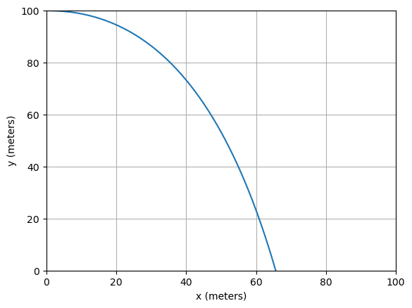
Consider an object being projected from the top of a tall building.
We know its initial position and speed in each direction and wish to predict its trajectory.

Projectile example - model#
In order to produce a model we need to decide which are the most important forces acting on the object:
gravity;
air resistance.
Note that gravity only acts in the negative \(y\) direction (not in the \(x\) direction), and always leads to a constant acceleration (\(g = 9.81 \, \mathrm{m}/\mathrm{s}^2\)).
Air resistance opposes the motion in both the \(x\) and \(y\) directions, and we will assume that the force is proportional to the speed in each direction (as we did in the free fall example in Lecture 12: Derivatives and differential equations).
Projectile example - equations#
Using the following notation
\(X(t)\) is the horizontal distance of the object at time \(t\)
\(Y(t)\) is the vertical distance of the object at time \(t\)
\(U(t)\) is the horizontal speed of the object at time \(t\)
\(V(t)\) is the vertical speed of the object at time \(t\)
The above model leads to the following two differential equations:
We also know, from the definition of speed, that
Projectile example - initial conditions#
In addition to the above 4 differential equations for the unknown speeds (\(U\) and \(V\)) and distances (\(X\) and \(Y\)) we also need to know the initial configuration of the system.
For example, when \(t = 0\):
\(U = 20\);
\(V = 0\);
\(X = 0\);
\(Y = 100\).
Note that we have dropped the units here for convenience, but those are implicit.
Projectile example - implementation#
def projectile(n, t0, tfinal):
    t = np.zeros([n + 1, 1])  # Initialise the array t
    U = np.zeros([n + 1, 1])  # Initialise the array U
    V = np.zeros([n + 1, 1])  # Initialise the array V
    X = np.zeros([n + 1, 1])  # Initialise the array X
    Y = np.zeros([n + 1, 1])  # Initialise the array Y

    ## define initial conditions
    t[0] = 0.0
    U[0] = 20.0
    V[0] = 0.0
    X[0] = 0.0
    Y[0] = 100.0

    ## define constants
    k = 0.2
    g = 9.81

    ## Calculate size of each interval
    dt = (tfinal - t0) / float(n)

    ## Take n steps of Euler’s method
    for i in range(n):
        U[i + 1] = U[i] + dt * (-k * U[i])
        V[i + 1] = V[i] + dt * (-k * V[i] - g)
        X[i + 1] = X[i] + dt * U[i]
        Y[i + 1] = Y[i] + dt * V[i]
        t[i + 1] = t[i] + dt

    return t, X, Y, U, V
Show code cell source
import numpy as np
from matplotlib import pyplot as plt

t0 = 0.0
tfinal = 6.0

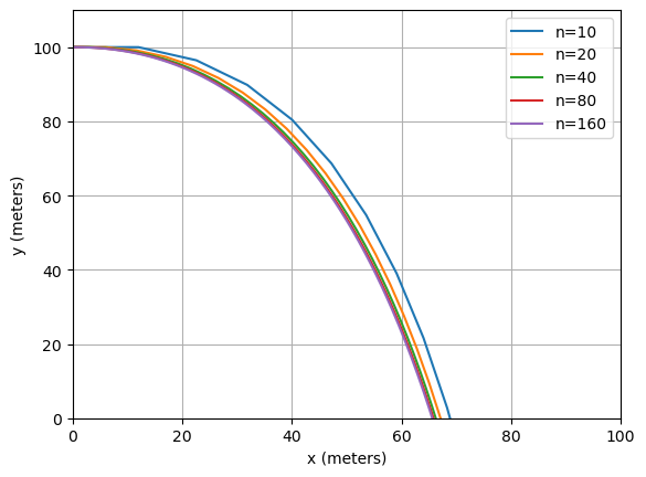
for n in [10, 20, 40, 80, 160]:
    t, X, Y, U, V = projectile(n, t0, tfinal)
    plt.plot(X, Y, label=f"{n=}")

plt.xlabel("x (meters)")
plt.ylabel("y (meters)")
plt.xlim(0.0, 100.0)
plt.ylim(0.0, 110.0)
plt.legend()
plt.grid()
plt.show()

Systems of equations#
The above example shows how Euler’s method can be applied to a system of four differential equations.
In general, a system of four differential equations will take the form:
\[\begin{split} \begin{aligned} Y_1'(t) & = F_1(t, Y_1, Y_2, Y_3, Y_4) \\ Y_2'(t) & = F_2(t, Y_1, Y_2, Y_3, Y_4) \\ Y_3'(t) & = F_3(t, Y_1, Y_2, Y_3, Y_4) \\ Y_4'(t) & = F_4(t, Y_1, Y_2, Y_3, Y_4). \end{aligned} \end{split}\]How does this relate to the projectile example above?
It is possible to apply Euler’s method or the midpoint method to apply Euler’s method or the midpoint method to a general system such as this:
These examples may look quite complex at first but they are simply applying the same techniques to systems of differential equations rather than a single differential equation.
Solution using Euler’s method#
Consider the following system of differential equations:
\[\begin{split} \vec{y}'(t) = A \vec{y}(t), \quad \text{ subject to } \quad \vec{y}(0) = \begin{pmatrix} 0 \\ 1 \end{pmatrix}, \end{split}\]where \(\vec{y}(t) = \begin{pmatrix} y_1(t) \\ y_2(t) \end{pmatrix}\) and \(A = \begin{pmatrix} -1 & 1 \\ 1 & -2 \end{pmatrix}\).
Approximate the solution using 2 steps of Euler’s method with \(\mathrm{d}t = 0.5\).
This gives
\[\begin{split} \begin{aligned} \vec{y}^{(i+1)} & = \vec{y}^{(i)} + \mathrm{d}t \begin{pmatrix} -1 & 1 \\ 1 & -2 \end{pmatrix} \vec{y}^{(i)} \\ t^{(i+1)} & = t^{(i)} + \mathrm{d}t. \end{aligned} \end{split}\]Writing this in component form and using python notation, this gives the following at each step:
y1[i+1] = y1[i] + 0.5 * (-y1[i] + y2[i])
y2[i+1] = y2[i] + 0.5 * (y1[i] - 2 * y2[i])
t[i+1] = t[i] + 0.5
or
y[i + 1, :] = y[i, :] + 0.5 * A @ y[i, :]
t[i+1] = t[i] + 0.5
Discussion#
Many useful models take the form of a single differential equation.
However, many important models require systems of coupled differential equations to be solved.
In the latter case we may generalise the standard techniques, such as Euler’s method or the midpoint method, to get effective computational models.
Only 2 computational schemes have been introduced here (Euler and midpoint) - there are many more that we haven’t considered…
Further reading#
Wikipedia: Projectile motion
The slides used in the lecture are also available

