Lecture 15: Introduction to nonlinear equations#
The problem#
Given a continuous function \(f(x)\), the problem is to find a point \(x^*\) such that \(f(x^*) = 0\). That is, \(x^*\) is a solution of the equation \(f(x) = 0\) and is called a root of \(f(x)\).
Examples
The linear equation \(f(x) = a x + b = 0\) has a single solution at \(x^* = -\frac{b}{a}\).
The quadratic equation \(f(x) = a x^2 + b x + c = 0\) is nonlinear , but simple enough to have a known formula for the solutions
\[ x^* = \frac{-b \pm \sqrt{b^2 - 4ac}}{2a}. \]A general nonlinear equation \(f(x) = 0\) rarely has a formula like those above which can be used to calculate its roots.
It is also sometimes better to use a numerical method to solve an equation even if an exact formula exists:
the exact formula may have difficulties due to rounding errors;
the exact formula may be more expensive to compute.
Example problems#
The following three example problems will be used throughout this section to illustrate the properties of common methods for solving nonlinear equations.
Calculate the value of \(x = \sqrt{R}\), where \(R\) is some positive real number, without the direct use of any
sqrtfunction.Let \(f(x) = x^2 - R\).
The equations \(f(x) = 0\) implies that \(x^2 = R\), i.e. \(x = \pm \sqrt{R}\).
There are two solutions and the method should be able to distinguish between them.
The following formula allows the monthly repayments (\(M\)) on a compound interest mortgage (for a borrowing of \(P\)) to be calculated based upon an annual interest rate of \(r\)% and \(n\) monthly payments (more details).
\[ M = P \frac{\frac{r}{1200} \left(1 + \frac{r}{1200}\right)^n}{\left(1 + \frac{r}{12000}\right)^n - 1}. \]Suppose that we wish to work out how many monthly repayments of £1,000 would be required to repay a mortgage of £150,000 at an annual rate of 5%.
This would require us to solve \(f(n) = 0\) where \(f(n) = 1000 - 150000 \frac{\frac{5}{1200}(1+\frac{5}{1200})^n}{(1+\frac{5}{1200})^n - 1}\).
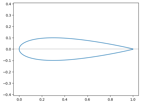
Consider the NACA0012 prototype wing section, which is often used for testing computational methods for simulating flows in aerodynamics:
Video source: https://youtu.be/wcahAqSFZ8k
The profile is given by
in which \(+\) gives the upper surface and \(-\) gives the lower surface.
Find the point \(x\) at which the thickness \(t\) of the aerofoil is \(0.1\), i.e. solve \(f(x) = 0\) where \(f(x) = y^+(x) - y^-(x) - 0.1\).
There will be two solutions for \(x\) for this value of \(t\).
Iterative methods#
Use the concept of iterative (or iterative improvement) again.
Given an initial estimate of the root \(x^{(0)}\), try to generate a better approximation \(x^{(1)}\) to the root.
Once \(x^{(1)}\) has been computed, it can be used to compute another estimate \(x^{(2)}\) in the same way (and so on…).
Generally, \(x^{(i)}\) is used to compute \(x^{(i+1)}\) (though other previous estimates may be used as well).
There are many methods for doing this.
Issues#
Does the iteration converge?
That is, will \(x^{(i+1)}\) be a better estimate than \(x^{(i)}\)?
How will we know if this is true or not?
If the iteration does converge then how quickly does this happen?
How should we decide when to stop the iterative procedure?
Bisection method#
The simplest method for solving \(f(x) = 0\), finding \(x^*\) such that \(f(x^*) = 0\), is known as the bisection method.
Assume for now that two points \(x_L\) and \(x_R\) are known for which
\[ f(x_L) f(x_R) < 0 \]i.e., the function evaluations at these points are of opposite sign.
If \(f\) is continuous then this implies that there must be at least one root \(x^*\) in the interval \((x_L, x_R)\). There may be more than one root.
The algorithm#
Consider the point \(x_C = (x_L + x_R) / 2\) and find \(f(x_C)\).
If \(f(x_C) = 0\), then \(x^* = x_C\) and we can stop.
If \(f(x_L) f(x_C) < 0\), then \(x^* \in (x_L, x_C)\).
If \(f(x_C) f(x_R) < 0\), then \(x^* \in (x_C, x_R)\).
Replace the interval (also termed bracket) \((x_L, x_R)\) with the new interval containing \(x^*\).
Note that in one step the length of the interval containing \(x^*\) has been halved.
Repeat this process until \(x_R - x_L < TOL\), where \(TOL\) is a user-supplied value, i.e. repeat until the bracket is sufficiently small.
Convergence analysis#
Assume that \(k\) steps are taken from an initial bracket \((a, b)\).
At each step the bracketing interval is halved.
So, after \(k\) steps the length of the interval will be \(\dfrac{b-a}{2^k}\).
For large \(b-a\) (a large initial bracket) or small \(TOL\) (high accuracy required) \(k\) will be large.
Note that once \(x_R - x_L < TOL\), we can estimate \(x^* = (x_L + x_R)/2\), in which case the absolute error will be at most \(\frac{1}{2} TOL\).
Example 1#
Use the bisection method to calculate \(\sqrt{2}\) with an error of less than \(10^{-4}\).
Use \(R = 2\), so \(f(x) = x^2 - 2\), which gives \(x^* = \sqrt{2}\).
Set the initial bracket to be \([a, b] = [0, 2]\) and the error tolerance to be \(TOL = 10^{-4}\).
---------------------------------------------------------------------------
AttributeError                            Traceback (most recent call last)
Cell In[3], line 40
     37 import pandas as pd
     39 df = pd.DataFrame(data, columns=headers)
---> 40 df.style.hide_index().set_caption("Results of bisection method on example 1")

AttributeError: 'Styler' object has no attribute 'hide_index'
Note that
choosing \([a, b] = [-2, 0]\) results in \(x^* = -1.4142\);
if \([a, b]\) brackets both roots, \(\pm \sqrt{R}\), then \(f(x_L) f(x_R) > 0\) and the bisection method cannot start.
Which roots, if any will the following initial intervals converge to?
Example 2#
Use the bisection method to calculate the number of monthly repayments of £1,000 that are required to repay a mortgage of £150,000 at an annual rate of 5%.
It is clear that 1 monthly repayment (\(n=1\)) will not be sufficient, whilst we should try a very large value of \(n\) to try to bracket the correct solution.
We converges to a solution of \(x^* = 235.9\) after 13 iterations.
Note that if we do not try a sufficiently large value for \(n\) for the upper range of the bracketing interval the method will fail.
Example 3#
Use the bisection method to find the points at which the thickness of the NACA0012 aerofoil is 0.1 with an error of less than \(10^{-4}\).
It can be seen that \(0 \le x^* \le 1\) but there are two solutions in this interval, so try \([x_L, x_R] = [0.5, 1]\) as the initial bracket.
This gives the root as \(x^* \approx 0.7652\) after 12 iterations.
Note that:
taking \([x_L, x_R] = [0, 0.5]\) gives the other root \(x^* \approx 0.0339\);
taking \([x_L, x_R] = [0, 1]\) or \([x_L, x_R] = [0.1, 0.6]\) would fail to give an initial bracket.
Weaknesses of the bisection algorithm#
Bisection is a reliable method for finding solutions of \(f(x) = 0\) provided an initial bracket can be found.
It is far from perfect however:
finding an initial bracket is not always easy;
it can take a very large number of iterations to obtain an accurate answer;
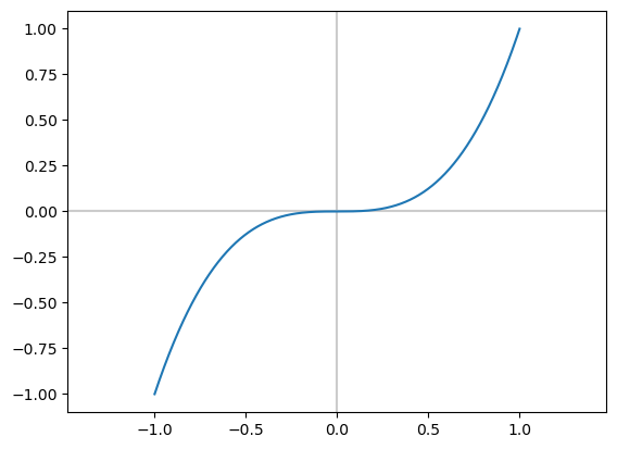
it can never find solutions of \(f(x) = 0\) for which \(f\) does not change sign.
For example:
Newton’s method#
Newton’s method (or the Newton-Raphson iteration) is an alternative algorithm for solving \(f(x) = 0\).
On the positive side:
it does not require an initial bracket - just an initial iterate;
it converges much more quickly than bisection;
it can solve problems where the solution is also a turning point (see previous example).
On the negative side:
it is not guaranteed to converge (unlike bisection with a good initial bracket).
Graphical derivation of Newton’s method#
\(x^{(i+1)}\) is computed by projecting the slope at \(x^{(i)}\), \(f'(x^{(i)})\), on to the \(x\)-axis, giving
Notes#
The formula \(x^{(i+1)} = x^{(i)} - \frac{f(x^{(i)})}{f'(x^{(i)})}\) requires an initial guess at the solution: \(x^{(0)}\).
In order to apply Newton’s method we need to be able to compute an expression for the derivative of \(f(x)\):
this may not always be possible or easy;
in the examples that follow we will make use of the formula:
\[ f(x) = x^n \Rightarrow f'(x) = n x^{n-1}, \]which is true for any \(n \neq 0\).
There are variants of Newton’s method that allow the derivative to be approximated: we will return to these later.
Examples#
Write out an expression for the Newton iteration for each of the following functions \(f(x)\) and then carry out 2 iterations using the resulting iteration and the given initial value \(x^{(0)}\).
\(f(x) = x^2 - 5\) with \(x^{(0)} = 2\).
This gives \(f'(x) = 2x\) so the iterative formula is
\[ x^{(i+1)} = x^{(i)} - \frac{(x^{(i)})^2 - 5}{2 x^{(i)}} = \frac{(x^{(i)})^2 + 5}{2 x^{(i)}}. \]This gives
\[\begin{split} \begin{aligned} x^{(1)} & = \frac{2^2 + 5}{2 \times 2} = \frac{9}{4} = 2.25 \\ x^{(2)} & = \frac{(\frac{9}{4})^2 + 5}{2 \times \frac{9}{4}} = \frac{161}{72} \approx 2.23611 \end{aligned} \end{split}\](Note \(\sqrt{5} = 2.23607\))
\(f(x) = x^3 - 2x - 5\) with \(x^{(0)} = 2\). (homework)
\(f(x) = x^3 - 2\) with \(x^{(0)} = 1\). (homework)
Summary#
Bisection approach is a simple and reliable algorithm for solving a nonlinear equation.
An appropriate initial bracket must be found - some searching may be required to locate one.
The analysis shows that the method is not very fast.
Newton’s method is an alternative approach:
it does not require an initial bracket - just an initial iterate;
it converges much more quickly than bisection;
it can solve problems where the solution is also a turning point;
We will discuss some drawbacks of Newton’s method next time…
Further reading#
Maths is fun: Quadratic equation
John D Cook, “The quadratic formula and low-precision arithmetic”
Wikipedia: Root finding algorithms
Wikipedia: Bisection method
Wikipedia: Newton’s method
X-engineer: Bisection method for root finding
The slides used in the lecture are also available