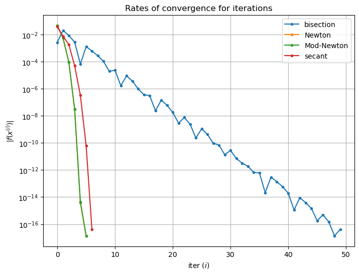
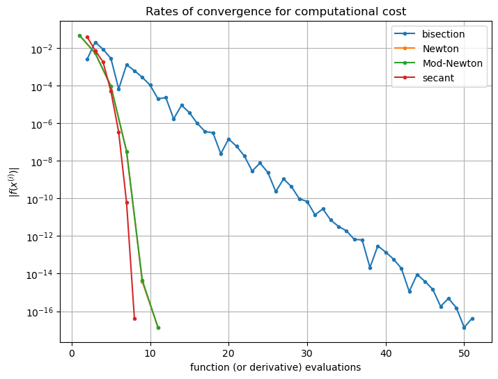
Lecture 17: Quasi-Newton methods

The problem

Given a continuous function \(f(x)\), the problem is to find a point \(x^*\) such that \(f(x^*) = 0\). That is, \(x^*\) is a solution of the equation \(f(x) = 0\) and is called a root of \(f(x)\).

Recall Newton’s method:

\[x^{(i+1)} = x^{(i)} - \frac{f(x^{(i)})}{f'(x^{(i)})}\]

def newton(f, df, x0, tol=1.0e-10):
    x = x0

    while abs(f(x)) > tol:
        x = x - f(x) / df(x)

    return x

Newton’s method requires function and it’s derivative.

This may not be possible since:

• \(f(x)\) may be a “black box”

• the formula for \(f(x)\) may be known but difficult to differentiate

• the derivative maybe very expensive to evaluate

Approximating f’(x)

Let’s approximate \(f'(x)\) like we approximated \(y'(t)\) when solving a differential equation!

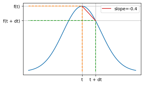
Modified Newton’s method

• Recall that \(f'(x) = \lim_{\mathrm{d}x \to 0} \frac{f(x + \mathrm{d}x) - f(x)}{\mathrm{d}x}\).

• Hence we can choose a small value for \(\mathrm{d}x\) (how small?) and approximate:

  \[ f'(x) \approx \frac{f(x + \mathrm{d}x) - f(x)}{\mathrm{d}x}. \]

• This modified-Newton method then becomes

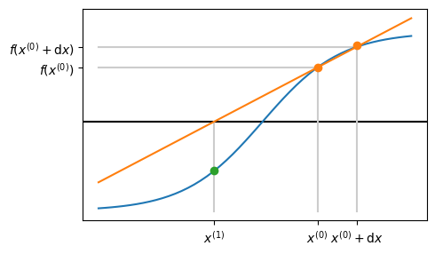
  \[ x^{(i+1)} = x^{(i)} - \frac{\mathrm{d}x \times f(x^{(i)})}{f(x^{(i)} + \mathrm{d}x) - f(x^{(i)})}. \]

def modified_newton(f, x0, dx, tol=1.0e-10):
    x = x0

    while abs(f(x)) > tol:
        df = (f(x + dx) - f(x)) / dx  # two extra evaluations of f
        # per iteration
        x = x - f(x) / df

    return x

def modified_newton2(f, x0, dx, tol=1.0e-10):
    x = x0
    fx = f(x)

    while abs(fx) > tol:
        df = (f(x + dx) - fx) / dx  # one extra evaluations of f
        # per iteration
        x = x - fx / df
        fx = f(x)  # one original evaluation of f per iteration

    return x

Graphical representation of modified Newton

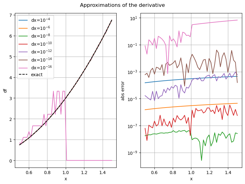
How to choose \(\mathrm{d}x\)?

Smaller - more accurate approximation

Large - too small and we will have rounding problems (subtracting two similar numbers)

Example

• When \(f(x) = x^3\) then \(f'(x) = 3 x^2\).

• Hence, at \(x_0 = 1\), \(f(x_0) = 1\) and \(f'(x_0) = 3\).

• Consider what happens when we approximate this with python, using finite values for \(\mathrm{d}x\).

Simple approximation of a derivative using floating point arithmetic

dx	approx	abs error	rel error
1.000000e-04	3.000300	3.000100e-04	1.000033e-04
1.000000e-06	3.000003	2.999798e-06	9.999326e-07
1.000000e-08	3.000000	3.972048e-09	1.324016e-09
1.000000e-10	3.000000	2.482211e-07	8.274037e-08
1.000000e-12	3.000267	2.667017e-04	8.890058e-05
1.000000e-14	2.997602	2.397834e-03	7.992778e-04
1.000000e-16	0.000000	3.000000e+00	1.000000e+00

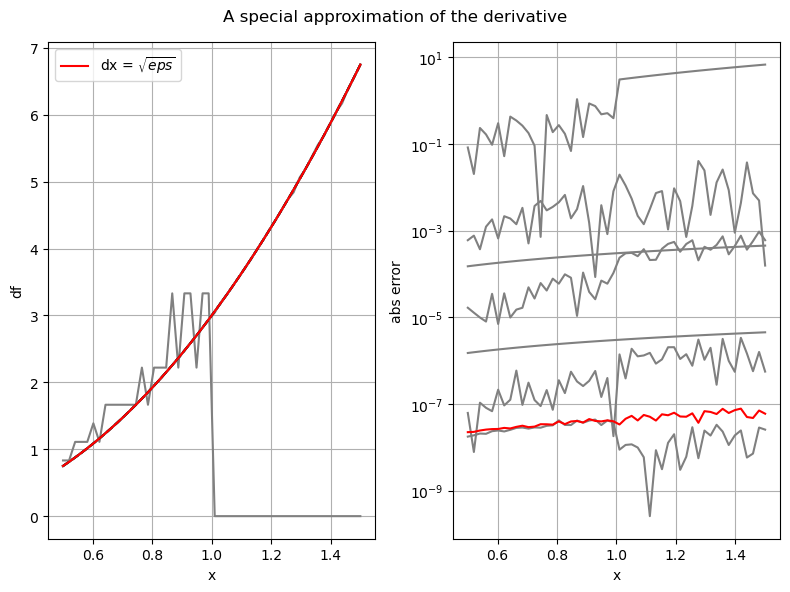
A special choice!

• Recall the definition of machine precision/unit roundoff from Lecture 3.

• The modified Newton method uses \(\mathrm{d}x = \sqrt{eps}\).

eps = np.finfo(np.double).eps
dx = np.sqrt(eps)

print(f"{eps=} {dx=}")

eps=2.220446049250313e-16 dx=1.4901161193847656e-08

Example

Recall the NACA0012 aerofoil example:

def f_naca0012(x):
    t = 0.1

    yp = (
        -0.1015 * x**4 + 0.2843 * x**3 - 0.3516 * x**2 - 0.126 * x + 0.2969 * np.sqrt(x)
    )
    f = yp - 0.5 * t

    return f

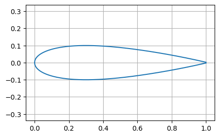
Starting from \(x^{(0)} = 1\) with \(TOL = 10^{-4}\), we get the root as \(x^* \approx 0.765789\) after 2 iterations for the NACA0012 aerofoil example (Same as Newton!):

modified_newton_with_table(f_naca0012, x0=1.0, tol=1.0e-4)

iter	x	f(x)
0	1.000000	-0.047900
1	0.795168	-0.005392
2	0.765789	-0.000096

Starting from \(x^{(0)} = 0.1\) with \(TOL = 10^{-4}\), we get the root as \(x^* \approx 0.033863\) after 5 iterations for the second solution to the NACA0012 aerofoil example (Same as Newton!).

modified_newton_with_table(f_naca0012, x0=0.1, tol=1.0e-4)

iter	x	f(x)
0	0.100000	0.028046
1	0.000278	-0.045086
2	0.005413	-0.028849
3	0.020693	-0.010046
4	0.031958	-0.001300
5	0.033863	-0.000024

The secant method

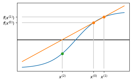
Can we use a similar derivative approximation but avoid the extra function evaluation?

Recall modified-Newton method:

\[ x^{(i+1)} = x^{(i)} - \frac{\mathrm{d}x \times f(x^{(i)})}{f(x^{(i)} + \mathrm{d}x) - f(x^{(i)})}. \]

Now with \(\mathrm{d}x = x^{(i)} - x^{(i-1)}\) becomes

\[ x^{(i+1)} = x^{(i)} - \frac{(x^{(i)} - x^{(i-1)}) \times f(x^{(i)})}{f(x^{(i)}) - f(x^{(i-1)})}. \]

def secant(f, x0, x1, tol=1.0e-10):
    # two initial function evaluations
    f0 = f(x0)
    f1 = f(x1)

    while abs(f1) > tol:
        # compute derivative approximation
        df = (f1 - f0) / (x1 - x0)
        # update x
        x2 = x1 - f1 / df

        # update other variables
        x0, f0 = x1, f1
        x1, f1 = x2, f(x2)  # one evaluation of f per iteration

    return x1

A geometric interpretation

Numerical examples

• The naca0012 example starting from 1 and 0.9 to a tolerance of \(10^{-4}\) gives the solution as \(x^* \approx 0.765264\) after 3 iterations (one more than Newton!)

secant_with_table(f_naca0012, x0=1.0, x1=0.9, tol=1.0e-4)

iter	x0	f(x0)	x1	f(x1)
0	1.000000	-0.047900	0.900000	-0.025871
1	0.900000	-0.025871	0.782556	-0.003095
2	0.782556	-0.003095	0.766598	-0.000239
3	0.766598	-0.000239	0.765264	-0.000003

Starting from \(x^{(0)} = 0.0\) and \(x^{(1)} = 0.1\) with \(TOL = 10^{-4}\), we get the root as \(x^* \approx 0.033870\) after 5 iterations for the second solution to the NACA0012 aerofoil example (Same as Newton!).

secant_with_table(f_naca0012, x0=0.0, x1=0.1, tol=1.0e-4)

iter	x0	f(x0)	x1	f(x1)
0	0.000000	-0.050000	0.100000	0.028046
1	0.100000	0.028046	0.064065	0.015706
2	0.064065	0.015706	0.018327	-0.012232
3	0.018327	-0.012232	0.038352	0.002810
4	0.038352	0.002810	0.034611	0.000465
5	0.034611	0.000465	0.033870	-0.000019

Turning points?

def f_turning(x):
    return (x - 1) ** 2


secant_with_table(f_turning, x0=4.0, x1=3.0, tol=1.0e-4)

iter	x0	f(x0)	x1	f(x1)
0	4.000000	9.000000	3.000000	4.000000
1	3.000000	4.000000	2.200000	1.440000
2	2.200000	1.440000	1.750000	0.562500
3	1.750000	0.562500	1.461538	0.213018
4	1.461538	0.213018	1.285714	0.081633
5	1.285714	0.081633	1.176471	0.031142
6	1.176471	0.031142	1.109091	0.011901
7	1.109091	0.011901	1.067416	0.004545
8	1.067416	0.004545	1.041667	0.001736
9	1.041667	0.001736	1.025751	0.000663
10	1.025751	0.000663	1.015915	0.000253
11	1.015915	0.000253	1.009836	0.000097

Other problems

Even more care is required to avoid divide by zero errors

# equal function values at x0 and x1
secant(f_turning, x0=4.0, x1=-2.0, tol=1.0e-4)

---------------------------------------------------------------------------
ZeroDivisionError                         Traceback (most recent call last)
Cell In[23], line 2
      1 # equal function values at x0 and x1
----> 2 secant(f_turning, x0=4.0, x1=-2.0, tol=1.0e-4)

Cell In[17], line 10, in secant(f, x0, x1, tol)
      8 df = (f1 - f0) / (x1 - x0)
      9 # update x
---> 10 x2 = x1 - f1 / df
     12 # update other variables
     13 x0, f0 = x1, f1

ZeroDivisionError: float division by zero

# too small tolerance means x0 = x1!
secant(f_turning, x0=4.0, x1=3.0, tol=1.0e-50)

---------------------------------------------------------------------------
ZeroDivisionError                         Traceback (most recent call last)
Cell In[24], line 2
      1 # too small tolerance means x0 = x1!
----> 2 secant(f_turning, x0=4.0, x1=3.0, tol=1.0e-50)

Cell In[17], line 8, in secant(f, x0, x1, tol)
      4 f1 = f(x1)
      6 while abs(f1) > tol:
      7     # compute derivative approximation
----> 8     df = (f1 - f0) / (x1 - x0)
      9     # update x
     10     x2 = x1 - f1 / df

ZeroDivisionError: float division by zero

Exercise (hard!)

Find a periodic iteration for the secant method.

Summary

	Bisection	Newton’s method	Modified Newton	Secant
Simple algorithm	yes	yes	yes	yes
Starting values	bracket	one	one	two
Iterations	lots	normally fewer	similar to Newton	similar to Newton
Function evals	one per iteration	f and df per iteration	two per iteration	one per iteration
Convergence	with good bracket	not always	not always	not always
Turing point roots	no	slower	slower	slower
Use of derivative	no	yes	no	no