This week#
An introduction to nonlinear solvers#
Why do we need nonlinear solvers?#
Given a continuous function \(f(x)\), the problem is to find a point \(x^*\) such that \(f(x^*) = 0\). That is, \(x^*\) is a solution of the equation \(f(x) = 0\) and is called a root of \(f(x)\).
Examples#
The linear equation \(f(x) = a x + b = 0\) has a single solution at \(x^* = -\frac{b}{a}\).
The quadratic equation \(f(x) = a x^2 + b x + c = 0\) is nonlinear , but simple enough to have a known formula for the solutions
\[ x^* = \frac{-b \pm \sqrt{b^2 - 4ac}}{2a}. \]A general nonlinear equation \(f(x) = 0\) rarely has a formula like those above which can be used to calculate its roots.
Example from two years ago’s exam paper#
We want to solve the quadratic equation
for large values of \(m\). The exact solutions are \(m\) and \(\frac{1}{m}\).
# implementation of quadratic formula
def quad(a, b, c):
    """
    Return the roots of the quadratic polynomial a x^2 + b x + c = 0.
    """
    d = np.sqrt(b * b - 4 * a * c)
    return (-b + d) / (2 * a), (-b - d) / (2 * a)
# test for m = 1e8
m = 1e8
roots = quad(1, -(m + 1 / m), 1)

print(f"{roots=}")
roots=(100000000.0, 1.4901161193847656e-08)
# absolute and relative errors
exact_roots = (m, 1 / m)

abs_error = (abs(roots[0] - exact_roots[0]), abs(roots[1] - exact_roots[1]))
rel_error = (abs_error[0] / m, abs_error[1] / (1 / m))

print(f"{abs_error=}")
print(f"{rel_error=}")
abs_error=(0.0, 4.901161193847656e-09)
rel_error=(0.0, 0.49011611938476557)
The need for implicit time stepping methods (1)#
Consider the differential equation
def rhs1(x, t):
    return -2 * x


def euler(x0, dt, T, rhs):
    # initialise memory
    n = int(T / dt)
    x = np.empty(n + 1)
    t = np.empty(n + 1)

    # starting values
    x[0] = x0
    t[0] = 0.0

    # do the time loop
    for j in range(n):
        x[j + 1] = x[j] + dt * rhs(x[j], t[j])
        t[j + 1] = t[j] + dt

    return x, t
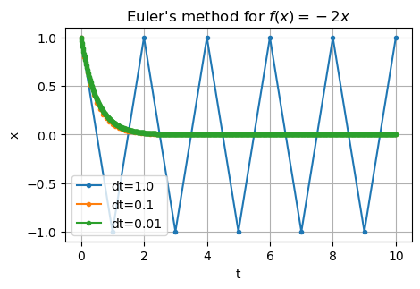
Recall explicit Euler says:
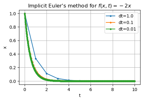
Consider instead the implicit Euler method:
We can’t simply evaluate the right hand side since we don’t know \(x^{(j+1)}\) yet!
For \(f(x, t) = -2x\), we can compute that
def implicit_euler(x0, dt, T):
    # initialise memory
    n = int(T / dt)
    x = np.empty(n + 1)
    t = np.empty(n + 1)

    # starting values
    x[0] = x0
    t[0] = 0.0

    # do the time loop
    for j in range(n):
        x[j + 1] = x[j] / (1.0 + 2.0 * dt)
        t[j + 1] = t[j] + dt

    return x, t
The need for implicit time stepping methods (2)#
Consider the differential equation
def rhs2(x, t):
    return -2 * x**3 * np.exp(-(1 - x**2))
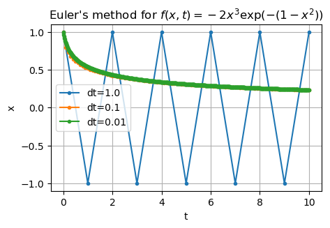
We might wish to use an implicit method, but how can we undo \(f\)??
Use a nonlinear solver!
Other difficult problems (1)#
The following formula allows the monthly repayments (\(M\)) on a compound interest mortgage (for a borrowing of \(P\)) to be calculated based upon an annual interest rate of \(r\)% and \(n\) monthly payments (more details).
Suppose that we wish to work out how many monthly repayments of £1,000 would be required to repay a mortgage of £150,000 at an annual rate of 5%.
This would require us to solve \(f(n) = 0\) where \(f(n) = 1000 - 150000 \frac{\frac{5}{1200}(1+\frac{5}{1200})^n}{(1+\frac{5}{1200})^n - 1}\).
Other difficult problems (2)#
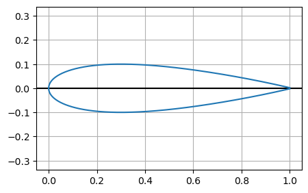
Consider the NACA0012 prototype wing section, which is often used for testing computational methods for simulating flows in aerodynamics
The profile is given by
in which \(+\) gives the upper surface and \(-\) gives the lower surface.
Find the point \(x\) at which the thickness \(t\) of the aerofoil is \(0.1\), i.e. solve \(f(x) = 0\) where \(f(x) = y^+(x) - y^-(x) - 0.1\).
There will be two solutions for \(x\) for this value of \(t\).
The bisection method#
Suppose the know there is a root \(x^*\) (\(f(x^*) = 0\)) between two end points \(a\) and \(b\)
Call \(c = \dfrac{a+b}{2}\), then the solution is either between \(a\) and \(c\) or between \(c\) and \(b\)
If the solution is between \(a\) and \(c\)
then go to step 1. with the end points as \(a\) and \(c\)
otherwise, go to step 1. with the end points as \(c\) and \(b\)
How can we tell that we have a solution between \(a\) and \(b\)?
How do we know we have a solution between \(a\) and \(b\)?#
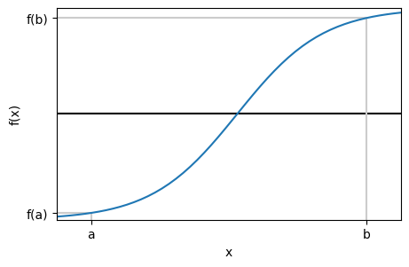
We test if \(f(a)\) and \(f(b)\) have opposite signs!
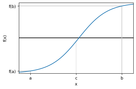
\(f(a)\) and \(f(c)\) have opposite signs so solution is between \(c\) and \(b\)!
# Simple bisection implementation
def bisection(func, a, b, tol=1.0e-10):
    # Starting values
    fa = func(a)
    fb = func(b)

    while b - a > tol:
        # Find new mid point
        c = (a + b) / 2
        fc = func(c)

        # if root is in left half of interval
        if fa * fc < 0.0:
            # move right end
            b = c
            fb = fc
        else:
            # otherwise,
            # move the left end
            a = c
            fa = fc

    return (a + b) / 2
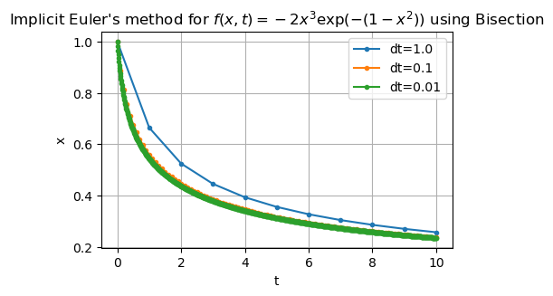
Implict Euler with bisection for the nonlinear solve#
Recall the differential equation:
Recall the implicit Euler method:
We cast this as a nonlinear equation to solve at each timestep: Find \(x^{(j+1)}\) such that
def implicit_euler(x0, dt, T):
    # initialise memory
    n = int(T / dt)
    x = np.empty(n + 1)
    t = np.empty(n + 1)

    # starting values
    x[0] = x0
    t[0] = 0.0

    # time loop
    for j in range(n):
        t[j + 1] = t[j] + dt

        # nonlinear function to solve each time step
        def F(xnew):
            return xnew - x[j] - dt * rhs2(xnew, t[j + 1])

        # perform the nonlinear solve
        x[j + 1] = bisection(F, -1.0, 1.0)

    return x, t
Example 2#
Use the bisection method to calculate the number of monthly repayments of £1,000 that are required to repay a mortgage of £150,000 at an annual rate of 5%.
It is clear that 1 monthly repayment (\(n=1\)) will not be sufficient, whilst we should try a very large value of \(n\) to try to bracket the correct solution.
M = 1000
P = 150000
r = 5


def f(x):
    return M - P * ((r / 1200) * (1 + r / 1200) ** x) / ((1 + r / 1200) ** x - 1)
| it | a | b | c | f(a) $\times$ f(c) | sign(f(a) $\times$ f(c)) | update |
|---|---|---|---|---|---|---|
| 0 | 1.00 | 1000.00 | 500.50 | -4.28e+07 | negative | b <- c |
| 1 | 1.00 | 500.50 | 250.75 | -5.19e+06 | negative | b <- c |
| 2 | 1.00 | 250.75 | 125.88 | 7.99e+07 | positive | a <- c |
| 3 | 125.88 | 250.75 | 188.31 | 8.06e+04 | positive | a <- c |
| 4 | 188.31 | 250.75 | 219.53 | 6.66e+03 | positive | a <- c |
| 5 | 219.53 | 250.75 | 235.14 | 8.26e+01 | positive | a <- c |
| 6 | 235.14 | 250.75 | 242.95 | -3.20e+01 | negative | b <- c |
| 7 | 235.14 | 242.95 | 239.04 | -1.45e+01 | negative | b <- c |
| 8 | 235.14 | 239.04 | 237.09 | -5.59e+00 | negative | b <- c |
| 9 | 235.14 | 237.09 | 236.12 | -1.06e+00 | negative | b <- c |
| 10 | 235.14 | 236.12 | 235.63 | 1.22e+00 | positive | a <- c |
| 11 | 235.63 | 236.12 | 235.87 | 2.73e-02 | positive | a <- c |
| 12 | 235.87 | 236.12 | 235.99 | -1.10e-02 | negative | b <- c |
| 13 | 235.87 | 235.99 | 235.93 | -4.62e-03 | negative | b <- c |
Example 3#
Use the bisection method to find the points at which the thickness of the NACA0012 aerofoil is 0.1 with an error of less than \(10^{-4}\).
It can be seen that \(0 \le x^* \le 1\) but there are two solutions in this interval, so try \([x_L, x_R] = [0.5, 1]\) as the initial bracket.
def f(x):
    yp = (
        -0.1015 * np.power(x, 4)
        + 0.2843 * np.power(x, 3)
        - 0.3516 * np.power(x, 2)
        - 0.126 * x
        + 0.2969 * np.sqrt(x)
    )
    t = 0.1
    return yp - 0.5 * t
| it | a | b | c | f(a) $\times$ f(c) | sign(f(a) $\times$ f(c)) | update |
|---|---|---|---|---|---|---|
| 0 | 0.50000 | 1.00000 | 0.75000 | 1.02152e-04 | positive | a <- c |
| 1 | 0.75000 | 1.00000 | 0.87500 | -5.54603e-05 | negative | b <- c |
| 2 | 0.75000 | 0.87500 | 0.81250 | -2.29940e-05 | negative | b <- c |
| 3 | 0.75000 | 0.81250 | 0.78125 | -7.63859e-06 | negative | b <- c |
| 4 | 0.75000 | 0.78125 | 0.76562 | -1.77701e-07 | negative | b <- c |
| 5 | 0.75000 | 0.76562 | 0.75781 | 3.49847e-06 | positive | a <- c |
| 6 | 0.75781 | 0.76562 | 0.76172 | 8.15966e-07 | positive | a <- c |
| 7 | 0.76172 | 0.76562 | 0.76367 | 1.73699e-07 | positive | a <- c |
| 8 | 0.76367 | 0.76562 | 0.76465 | 2.96088e-08 | positive | a <- c |
| 9 | 0.76465 | 0.76562 | 0.76514 | 2.11193e-09 | positive | a <- c |
| 10 | 0.76514 | 0.76562 | 0.76538 | -4.63408e-10 | negative | b <- c |
| 11 | 0.76514 | 0.76538 | 0.76526 | -3.40195e-11 | negative | b <- c |
| 12 | 0.76514 | 0.76526 | 0.76520 | 1.80650e-10 | positive | a <- c |
Example 4#
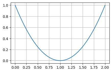
What about if the root is a turning point?
Summary#
Bisection |
|
|---|---|
Simple algorithm |
yes |
Starting values |
bracket |
Iterations |
lots |
Function evals |
one per iteration |
Convergence |
with good bracket |
Turing point roots |
no |
Use of derivative |
no |
Coursework clarifications#
Portfolio
Best 6 out of 8 sections count for your final grade
If you have full marks on the first 6 sections, the final two sections don’t count!
Final coursework
Deadline is Wed 18 Dec
Your submission should be an evaluated jupyter notebook (
.ipynb)
Recap of the bisection method#
Suppose the know there is a root \(x^*\) (\(f(x^*) = 0\)) between two end points \(a\) and \(b\)
Call \(c = \dfrac{a+b}{2}\), then the solution is either between \(a\) and \(c\) or between \(c\) and \(b\)
If the solution is between \(a\) and \(c\)
then go to step 1. with the end points as \(a\) and \(c\)
otherwise, go to step 1. with the end points as \(c\) and \(b\)
Bisection challenges (i)#
How to determine an initial bracket \((a, b)\)?
You need to have that \(f(a) \times f(b) < 0\) - i.e. there is a change of sign!
If \(f(x) \ge 0\) for all \(x\), bisection is not possible
If \(f(a) = 0\) or \(f(b) = 0\), then you have already found the route and you can stop!
Big brackets take a long time to get small
Bisection challenges (ii)#
How do you know you’ve still trapped the root?
If \(f(a) \times f(b) < 0\), then either \(f(a) \times f(c) < 0\), \(f(b) \times f(c) < 0\) or \(f(c) = 0\).
sign(\(f(a)\)) |
sign(\(f(b)\)) |
sign(\(f(c)\)) |
root between |
|---|---|---|---|
positive |
negative |
positive |
\(c\) and \(b\) |
positive |
negative |
negative |
\(a\) and \(c\) |
negative |
positive |
positive |
\(a\) and \(c\) |
negative |
positive |
negative |
\(c\) and \(b\) |
any |
any |
0 |
root is at \(c\) |
Newton’s method#
The bisection method needs lots of iterations because it doesn’t take into account the value of the function at the end points of the interval, only the sign
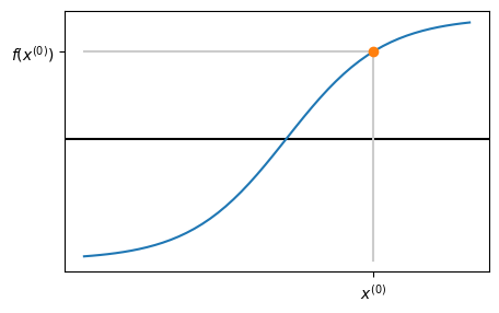
We consider now an alternative approach where we use the derivative of the function \(f\) to help improve the convergence rate!
Derivation of Newton’s method#
1. Evaluate function at current guess:#
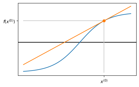
2. Trace tangent line using derivative#
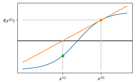
3. Next iterate \(x_1\) is where tangent line crosses \(x\)-axis#
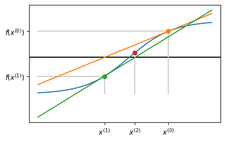
4. Go back to step 1. and repeat!#
So what’s the formula?#
Slope is
which rearranges to give
Python version#
def newton(f, df, x0, tol=1.0e-10):
    x = x0

    while abs(f(x)) > tol:
        x = x - f(x) / df(x)

    return x
def newton2(f, df, x0, tol=1.0e-10):
    x = x0
    fx = f(x)

    while abs(fx) > tol:
        x = x - fx / df(x)
        fx = f(x)  # only one function evaluation per loop

    return x
Examples of Newton’s method#
Starting from \(x^{(0)} = 1\) with \(TOL = 10^{-4}\), we get the root as \(x^* \approx 0.765789\) after 2 iterations for the NACA0012 aerofoil example:
Recall NACA0012 aerofoil example
def f(x):
    t = 0.1

    yp = (
        -0.1015 * np.power(x, 4)
        + 0.2843 * np.power(x, 3)
        - 0.3516 * np.power(x, 2)
        - 0.126 * x
        + 0.2969 * np.sqrt(x)
    )
    f = yp - 0.5 * t

    return f


def df(x):
    dy = (
        -4 * 0.1015 * np.power(x, 3)
        + 3 * 0.2843 * np.power(x, 2)
        - 2 * 0.3516 * x
        - 0.126
        + 0.2969 * 0.5 * np.power(x, -0.5)
    )
    f = dy

    return f
Starting from \(x^{(0)} = 1\) with \(TOL = 10^{-4}\), we get the root as \(x^* \approx 0.765789\) after 2 iterations for the NACA0012 aerofoil example:
| iter | x | f(x) |
|---|---|---|
| 0 | 1.000000 | -0.047900 |
| 1 | 0.795168 | -0.005392 |
| 2 | 0.765789 | -0.000096 |
Starting from \(x^{(0)} = 0.1\) with \(TOL = 10^{-4}\), we get the root as \(x^* \approx 0.033863\) after 5 iterations for the second solution to the NACA0012 aerofoil example.
| iter | x | f(x) |
|---|---|---|
| 0 | 0.100000 | 0.028046 |
| 1 | 0.000278 | -0.045086 |
| 2 | 0.005413 | -0.028849 |
| 3 | 0.020693 | -0.010046 |
| 4 | 0.031958 | -0.001300 |
| 5 | 0.033863 | -0.000024 |
Compare against a similar test with the bisection method - the Newton method is much faster!
| it | a | b | c | f(a) $\times$ f(c) | sign(f(a) $\times$ f(c)) | update |
|---|---|---|---|---|---|---|
| 0 | 0.50000 | 1.00000 | 0.75000 | 1.02152e-04 | positive | a <- c |
| 1 | 0.75000 | 1.00000 | 0.87500 | -5.54603e-05 | negative | b <- c |
| 2 | 0.75000 | 0.87500 | 0.81250 | -2.29940e-05 | negative | b <- c |
| 3 | 0.75000 | 0.81250 | 0.78125 | -7.63859e-06 | negative | b <- c |
| 4 | 0.75000 | 0.78125 | 0.76562 | -1.77701e-07 | negative | b <- c |
| 5 | 0.75000 | 0.76562 | 0.75781 | 3.49847e-06 | positive | a <- c |
| 6 | 0.75781 | 0.76562 | 0.76172 | 8.15966e-07 | positive | a <- c |
| 7 | 0.76172 | 0.76562 | 0.76367 | 1.73699e-07 | positive | a <- c |
| 8 | 0.76367 | 0.76562 | 0.76465 | 2.96088e-08 | positive | a <- c |
| 9 | 0.76465 | 0.76562 | 0.76514 | 2.11193e-09 | positive | a <- c |
| 10 | 0.76514 | 0.76562 | 0.76538 | -4.63408e-10 | negative | b <- c |
| 11 | 0.76514 | 0.76538 | 0.76526 | -3.40195e-11 | negative | b <- c |
| 12 | 0.76514 | 0.76526 | 0.76520 | 1.80650e-10 | positive | a <- c |
Zero derivative as a root#
We saw that the bisection method cannot deal with the situation where a root occurs at a turning point. That is,
\[ f(x^*) = f'(x^*) = 0. \]At first sight, it may appear that Newton’s method will struggle with such situations since \(x^{(i+1)} = x^{(i)} - \frac{f(x^{(i)})}{f'(x^{(i)})}\) would lead to \(\frac{0}{0}\) occurring when \(x^{(i)} = x^*\).
Fortunately, this is not a problem in practice and the iteration can still converge - although it converges more slowly than to a “simple root”.
Zero derivative as a root - example#
Find a solution of \(f(x) = 0\) using Newton’s method when
This has a solution \(x^* = 1\), however \(f'(x) = 2x - 2\), so \(f'(x^*) = 0\) when \(x = x^*= 1\).
def f(x):
    return (x - 1) ** 2


def df(x):
    return 2 * (x - 1)
newton_with_table(f, df, x0=4.0, tol=1.0e-4)
| iter | x | f(x) |
|---|---|---|
| 0 | 4.000000 | 9.000000 |
| 1 | 2.500000 | 2.250000 |
| 2 | 1.750000 | 0.562500 |
| 3 | 1.375000 | 0.140625 |
| 4 | 1.187500 | 0.035156 |
| 5 | 1.093750 | 0.008789 |
| 6 | 1.046875 | 0.002197 |
| 7 | 1.023438 | 0.000549 |
| 8 | 1.011719 | 0.000137 |
| 9 | 1.005859 | 0.000034 |
Problems with Newton’s methods#
When Newton’s method works it is a fast way of solving a nonlinear equation \(f(x) = 0\), but it does not always work.
Consider applying a Newton iteration to the function \(f(x) = x^3 + 2 x^2 + x + 1\) with \(x^{(0)} = 0\).
This gives \(f'(x) = 3 x^2 + 4 x + 1\). With \(x^{(0)} = 0\) this gives:
def f(x):
    return x**3 + 2 * x**2 + x + 1


def df(x):
    return 3 * x**2 + 4 * x + 1
/tmp/ipykernel_2201/2403100073.py:11: RuntimeWarning: divide by zero encountered in scalar divide
  x = x - f(x) / df(x)
/tmp/ipykernel_2201/475226614.py:2: RuntimeWarning: invalid value encountered in scalar add
  return x**3 + 2 * x**2 + x + 1
| iter | x | f(x) |
|---|---|---|
| 0 | 0.000000 | 1.000000 |
| 1 | -1.000000 | 1.000000 |
| 2 | -inf | nan |
We can also get cases where the iteration does not “blow up” but diverges slowly…
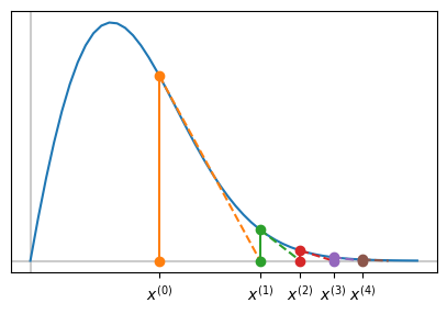
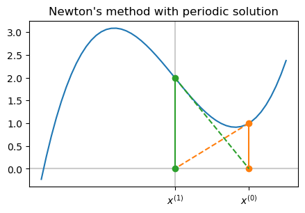
It is even possible for the iteration to simply cycle between two values repeatedly…
def f(t):
    return t**3 - 2 * t + 2


def df(t):
    return 3 * t**2 - 2
WARNING! Newton iteration has not converged. Too many iterations.
| iter | x | f(x) |
|---|---|---|
| 0 | 1.000000 | 1.000000 |
| 1 | 0.000000 | 2.000000 |
| 2 | 1.000000 | 1.000000 |
| 3 | 0.000000 | 2.000000 |
| 4 | 1.000000 | 1.000000 |
| 5 | 0.000000 | 2.000000 |
| 6 | 1.000000 | 1.000000 |
| 7 | 0.000000 | 2.000000 |
| 8 | 1.000000 | 1.000000 |
| 9 | 0.000000 | 2.000000 |
| 10 | 1.000000 | 1.000000 |
| 11 | 0.000000 | 2.000000 |
| 12 | 1.000000 | 1.000000 |
| 13 | 0.000000 | 2.000000 |
| 14 | 1.000000 | 1.000000 |
| 15 | 0.000000 | 2.000000 |
| 16 | 1.000000 | 1.000000 |
| 17 | 0.000000 | 2.000000 |
| 18 | 1.000000 | 1.000000 |
| 19 | 0.000000 | 2.000000 |
| 20 | 1.000000 | 1.000000 |
| 21 | 0.000000 | 2.000000 |
| 22 | 1.000000 | 1.000000 |
| 23 | 0.000000 | 2.000000 |
| 24 | 1.000000 | 1.000000 |
| 25 | 0.000000 | 2.000000 |
| 26 | 1.000000 | 1.000000 |
| 27 | 0.000000 | 2.000000 |
| 28 | 1.000000 | 1.000000 |
| 29 | 0.000000 | 2.000000 |
| 30 | 1.000000 | 1.000000 |
| 31 | 0.000000 | 2.000000 |
| 32 | 1.000000 | 1.000000 |
| 33 | 0.000000 | 2.000000 |
| 34 | 1.000000 | 1.000000 |
| 35 | 0.000000 | 2.000000 |
| 36 | 1.000000 | 1.000000 |
| 37 | 0.000000 | 2.000000 |
| 38 | 1.000000 | 1.000000 |
| 39 | 0.000000 | 2.000000 |
| 40 | 1.000000 | 1.000000 |
| 41 | 0.000000 | 2.000000 |
| 42 | 1.000000 | 1.000000 |
| 43 | 0.000000 | 2.000000 |
| 44 | 1.000000 | 1.000000 |
| 45 | 0.000000 | 2.000000 |
| 46 | 1.000000 | 1.000000 |
| 47 | 0.000000 | 2.000000 |
| 48 | 1.000000 | 1.000000 |
| 49 | 0.000000 | 2.000000 |
| 50 | 1.000000 | 1.000000 |
| 51 | 0.000000 | 2.000000 |
| 52 | 1.000000 | 1.000000 |
| 53 | 0.000000 | 2.000000 |
| 54 | 1.000000 | 1.000000 |
| 55 | 0.000000 | 2.000000 |
| 56 | 1.000000 | 1.000000 |
| 57 | 0.000000 | 2.000000 |
| 58 | 1.000000 | 1.000000 |
| 59 | 0.000000 | 2.000000 |
| 60 | 1.000000 | 1.000000 |
| 61 | 0.000000 | 2.000000 |
| 62 | 1.000000 | 1.000000 |
| 63 | 0.000000 | 2.000000 |
| 64 | 1.000000 | 1.000000 |
| 65 | 0.000000 | 2.000000 |
| 66 | 1.000000 | 1.000000 |
| 67 | 0.000000 | 2.000000 |
| 68 | 1.000000 | 1.000000 |
| 69 | 0.000000 | 2.000000 |
| 70 | 1.000000 | 1.000000 |
| 71 | 0.000000 | 2.000000 |
| 72 | 1.000000 | 1.000000 |
| 73 | 0.000000 | 2.000000 |
| 74 | 1.000000 | 1.000000 |
| 75 | 0.000000 | 2.000000 |
| 76 | 1.000000 | 1.000000 |
| 77 | 0.000000 | 2.000000 |
| 78 | 1.000000 | 1.000000 |
| 79 | 0.000000 | 2.000000 |
| 80 | 1.000000 | 1.000000 |
| 81 | 0.000000 | 2.000000 |
| 82 | 1.000000 | 1.000000 |
| 83 | 0.000000 | 2.000000 |
| 84 | 1.000000 | 1.000000 |
| 85 | 0.000000 | 2.000000 |
| 86 | 1.000000 | 1.000000 |
| 87 | 0.000000 | 2.000000 |
| 88 | 1.000000 | 1.000000 |
| 89 | 0.000000 | 2.000000 |
| 90 | 1.000000 | 1.000000 |
| 91 | 0.000000 | 2.000000 |
| 92 | 1.000000 | 1.000000 |
| 93 | 0.000000 | 2.000000 |
| 94 | 1.000000 | 1.000000 |
| 95 | 0.000000 | 2.000000 |
| 96 | 1.000000 | 1.000000 |
| 97 | 0.000000 | 2.000000 |
| 98 | 1.000000 | 1.000000 |
| 99 | 0.000000 | 2.000000 |
| 100 | 1.000000 | 1.000000 |
| 101 | 0.000000 | 2.000000 |
Summary#
Bisection |
Newton’s method |
|
|---|---|---|
Simple algorithm |
yes |
yes |
Starting values |
bracket |
one |
Iterations |
lots |
normally fewer |
Function evals |
one per iteration |
|
Convergence |
with good bracket |
not always |
Turing point roots |
no |
slower |
Use of derivative |
no |
yes |

