Today: A modelling example#
Tom Ranner
A model for the trajectory of an object#

Newton’s laws of motion#
Important in many computer games is the physics engine
This is often one of the computationally expensive parts of running a game
Models often derived by working out the forces on an object and applying Newton’s laws!
Force = mass \(\times\) acceleration
Newton’s 2nd law of motion states that the accerlation of an object in each direction is equal to the applied force in that direction divided by the mass of the object.
once we know the acceleration of the object, we can solve the differential equation to calculate the objects velocity and position…
Example - a projectile#
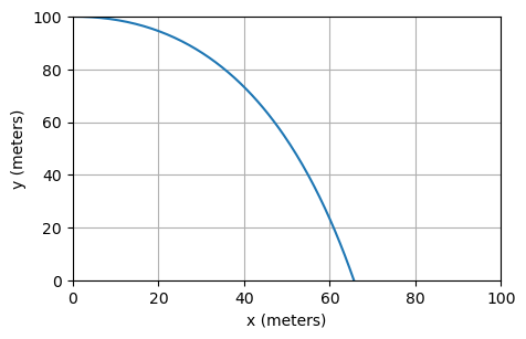
Consider an object being projected from the top of a tall building
We know its initial postion and speed in each direction and wish to predict is trajectory!

Project example - the model#
We consider a similar model to the freefall example from lecture 12.
The important forces are:
gravity acts in the negative \(y\) direction at a constant acceleration \(g = 9.81 \, \mathrm{m} / \mathrm{s}^2\)
air resistance acts in the opposite direction to way the projectile is moving - in both the \(x\) and \(y\) directions. We assume the size of the force is proportional to the speed is each direction
Projectile example - equations#
Using the following notation
\(X(t)\) is the horizontal distance of the object at time \(t\)
\(Y(t)\) is the vertical distance of the object at time \(t\)
\(U(t)\) is the horizontal speed of the object at time \(t\)
\(V(t)\) is the vertical speed of the object at time \(t\)
The above model leads to the following two differential equations:
We also know, from the definition of speed, that
Projectile example - initial conditions#
In addition to the 4 differential equations, we need 4 starting values.
For example at \(t = 0\),
(We’re not going to write down the units any more but they are still there!)
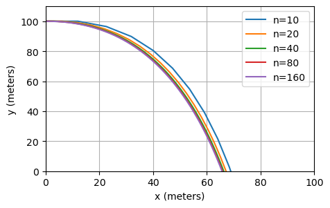
Projectile example - results#

Euler’s method for systems of equations#
In general, a system of four differential equations will take the form:
How does this relate to the projectile example above?
It is possible to apply Euler’s method or the midpoint method to apply Euler’s method or the midpoint method to a general system such as this
Solution using Euler’s method#
Consider the following system of differential equations:
where \(\vec{y}(t) = \begin{pmatrix} y_1(t) \\ y_2(t) \end{pmatrix}\) and \(A = \begin{pmatrix} -1 & 1 \\ 1 & -2 \end{pmatrix}\).
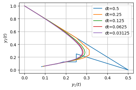
Approximate the solution using 2 steps of Euler’s method with \(\mathrm{d}t = 0.5\).
The Python version#
Using Python notation each time step would be given by
y1[i + 1] = y1[i] + 0.5 * (-y1[i] + y2[i])
y2[i + 1] = y2[i] + 0.5 * (y1[i] - 2 * y2[i])
t[i + 1] = t[i] + 0.5
or
y[i + 1, :] = y[i, :] + 0.5 * A @ y[i, :]
t[i + 1] = t[i] + 0.5
Python results#

What about errors?#
We can use the Euclidean norm as before to calculate the error against an exact solution:
| dt | abs. error | ratio |
|---|---|---|
| 0.500000 | 0.017606 | --- |
| 0.250000 | 0.008555 | 0.485941 |
| 0.125000 | 0.004219 | 0.493091 |
| 0.062500 | 0.002095 | 0.496579 |
| 0.031250 | 0.001044 | 0.498299 |
Summary#
Many useful models take the form of a single differential equation.
However, many important models require systems of coupled differential equations to be solved.
In the latter case we may generalise the standard techniques, such as Euler’s method or the midpoint method, to get effective computational models.
Only 2 computational schemes have been introduced here (Euler and midpoint) - there are many more that we haven’t considered…

