Today: Derivatives and dynamical models

Tom Ranner

Recap

Yesterday, we thought about the concept of rate of change

Speed is the rate of change of distance

Instantaneous speed is the limit of average speeds over shorter and shorter time periods

\[ S(t) = \lim_{\mathrm{d}t \to 0} \frac{D(t + \mathrm{d}t) - D(t)}{\mathrm{d}t}. \]

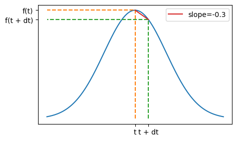
We also saw a geometric description:

More on graphs and derivatives

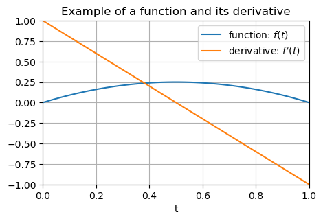
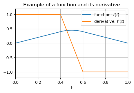
Example 1

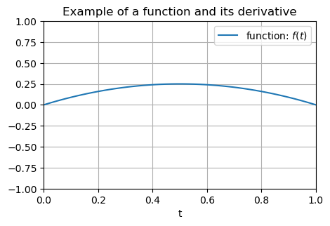
Example 1

Example 2

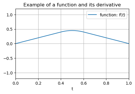
Example 2

Example 3

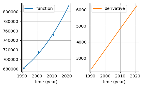
The population of Leeds over time (fitted):

Example 4

Climate data (fitted):

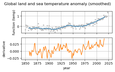
Data source: https://www.ncei.noaa.gov/access/monitoring/climate-at-a-glance/global/time-series

Differential equations

We have already seen \(S(t) = D'(t)\).

This is an example of a differential equation - an equation which involves one or more derivatives.

We have seen (and computationally solved!) one example:

\[ D'(t) = -(t - 1.0) (t + 0.5) \text{ where } D(0) = 0. \]

An object in free fall

Consider a simple model for an object falling from a large height, based on two assumptions:

1. all objects are attracted downward with an acceleration due to gravity of \(9.81\, \mathrm{m} / \mathrm{s}^2\)

2. air resistance causes an object to decelerate in proportion to its spead

What is the net acceleration on the object

Acceleration is the rate of change of speed! \(a(t) = S'(t)\)

A positive value for \(a(t)\) means that the speed is increasing whilst a negative value means that speed is decreasing.

We can write the downwards acceleration as

\[ a(t) = g - k S(t) \]

(here \(S(t)\) is the downwards speed)

So we have the differential equation:

\[ S'(t) = g - k S(t). \]

How can we solve this equation

Try to do the same as last lecture, split the time interval into small time interval and assume everything is constant on each time interval.

We know that

\[ S'(t) = \lim_{\mathrm{d}t \to 0} \frac{S(t + \mathrm{d}t) - S(t)}{\mathrm{d}t} \approx \frac{S(t+ \mathrm{d}t) - S(t)}{\mathrm{d}t} \]

for a small value of \(\mathrm{d}t\).

Hence we can iterate

\[ S(t + \mathrm{d}t) = S(t) + \mathrm{d}t (g - k S(t)). \]

Python algorithm

def freefall(n):
    """Input: n number of timesteps"""

    tfinal = 50.0  # Select the final time
    g = 9.81  # acceleration due to gravity (m/s)
    k = 0.2  # air resistance coefficient

    # initialise time and speed arrays array
    t = np.empty([n + 1, 1])
    s = np.empty([n + 1, 1])
    s[0], t[0] = 0.0, 0.0  # set initial conditions

    dt = (tfinal - t[0]) / n  # calculate step size

    # take n time steps, in which it is assumed that the acceleration
    # is constant in each small time interval
    for i in range(n):
        t[i + 1] = t[i] + dt
        s[i + 1] = s[i] + dt * (g - k * s[i])

    return t, s

Python algorithm results

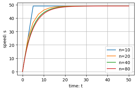
This approach works for any differential equation and is called Euler’s method

Euler’s method

An approach that works for any differential equation involving just a single derivative:

\[ y'(t) = f(t, y(t)) \quad \text{subject to the initial condition} \quad y(t_0) = y_0. \]

General form:

\[ y'(t) = f(t, y(t)) \quad \text{subject to the initial condition} \quad y(t_0) = y_0. \]

Examples

\[y'(t) = -(t-1.0)(t-0.5) \quad\text{and}\quad y(0) = 0\]

\[y'(t) = g - k y(t) \quad\text{and}\quad y(0) = 0\]

\[y'(t) = -(y(t))^2 + \frac{1}{t} \quad\text{and}\quad y(1) = 2\]

General algorithm

For differential equations in our general form, we have the following algorithm:

1. Set initial values for \(t^{(0)}\) and \(y^{(0)}\)

2. Loop over all time steps, until the final time, updaing using the formulae:

   \[\begin{split} \begin{aligned} y^{(i+1)} & = y^{(i)} + \mathrm{d}t f(t^{(i)}, y^{(i)}) \\ t^{(i+1)} & = t^{(i)} + \mathrm{d}t. \end{aligned} \end{split}\]

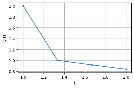
Example

Take three steps of Euler’s method to approximate the solution of

\[ y'(t) = -(y(t))^2 + \frac{1}{t} \text{ subject to the initial condition } y(1) = 2 \]

for \(1 \le t \le 2\).

Summary

• Given the graph of \(y(t)\) it is possible to sketch the graph of \(y'(t)\) (with some care!).

• Computational models which involve dynamic processes usually involve the use of derivatives.

• An equation which includes a derivative is known as a differential equation.

• To solve a differential equation it is necessary to know some information about the solution at some starting point (e.g. initial distance travelled, initial speed, population at a given point in time, etc.).

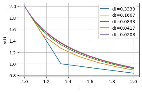
• One computational approach to solve such equations is Euler’s method - which gets more accurate with more sub-intervals used.