Today: Introduction to dynamic problems

Tom Ranner

Static vs dynamic problems

Examples so far have focussed on static problems that don’t change in time:

Static vs dynamic problems

There are many other problems that require models to change in time, that is the models are dynamic:

Rates of change

Suppose we know that a person is walking at constant 3 meters per second (m/s) - what does that mean?

So how far will they travel in:

• \(0.1\) seconds?

• \(0.01\) seconds?

• \(0.001\) seconds?

• \(10^{-6}\) seconds?

What does this tell us about speed?

\[ \text{Distance travelled} = \text{speed} \times \text{time} \]

That is, $\( \text{speed} = \dfrac{\text{distance travelled}}{\text{time}} \)$

Equivalently, $\( \text{speed} = \dfrac{(\text{distance at end}) - (\text{distance at start})}{\text{time}}. \)$

The derivative as a rate of change

What if the object’s speed was not constant? For example, \(S(t) = -(t-1.0)(t+0.5)\).

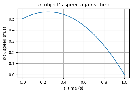
How far would the object travel in one second now? – with difficulty :(

We could consider each tenth of a second separately and estimate the distance covered at each tenth (assuming the \(s\) is approximately constant in each interval):

D, t = 0.0, 0.0
for i in range(10):
    D = D + 0.1 * S(t)
    t = t + 0.1

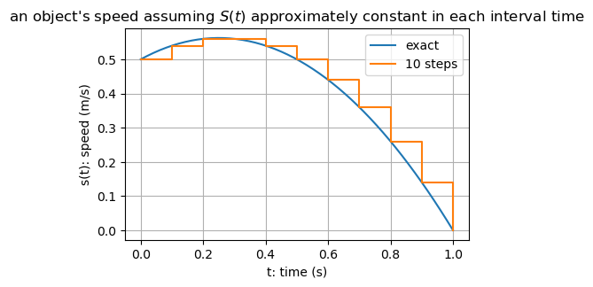
We could consider each hundredth of a second separately and estimate the distance covered at each hundredth (assuming the \(s\) is approximately constant in each interval):

D, t = 0.0, 0.0
for i in range(100):
    D = D + 0.01 * S(t)
    t = t + 0.01

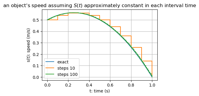
We could consider each thousandth of a second separately and estimate the distance covered at each thousandth (assuming the \(s\) is approximately constant in each interval):

D, t = 0.0, 0.0
for i in range(1000):
    D = D + 0.001 * S(t)
    t = t + 0.001

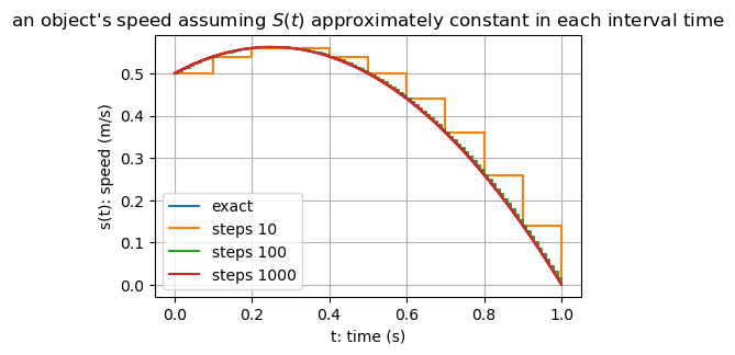
What values do we get?

Total distance as a function of number of steps

	# intervals	increment size dt	total distance
0	10	0.100000	0.440000
1	100	0.010000	0.419150
2	1000	0.001000	0.416916
3	10000	0.000100	0.416692
4	100000	0.000010	0.416669

… we appear to be converging to an answer in the limit as \(\mathrm{d}t \to 0\)…

So what’s going on

At any instant of time, the speed is the rate of change in distance:

\[ \text{speed} = \dfrac{\text{change in distance}}{\text{time}} \]

so

\[ \text{change in distance} = \text{time} \times \text{speed} \]

Mathematically speaking

Call the speed \(S(t)\) and distance \(D(t)\):

\[ S(t) = \frac{D(t + \mathrm{d}t) - D(t)}{\mathrm{d}t} \]

In fact, to obtain a converged answer, we must take smaller and smaller choices for \(\mathrm{d}t\):

\[ S(t) = \lim_{\mathrm{d}t \to 0} \frac{D(t + \mathrm{d}t) - D(t)}{\mathrm{d}t} \]

We say that speed, \(S(t)\), is the derivative of distance, \(D(t)\), with respect to time and write \(S(t) = D'(t)\).

A graphical interpretation

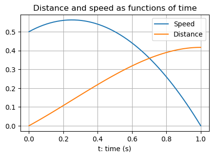
We see the gradient (slope) of the orange curve is the value of the blue curve.

The derivative as a gradient

What is the gradient of a line?

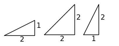
The equation of a straight line with slope \(m\) is given by

\[ y(t) = m t + c. \]

Slope of a curve

What is the gradient of a curve?

Well… the gradient of the straight-line approximation (chord) for a small step is

\[ \frac{y(t + \mathrm{d}t) - y(t)}{\mathrm{d}t}. \]

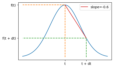
What about reducing \(\mathrm{d}t\)?

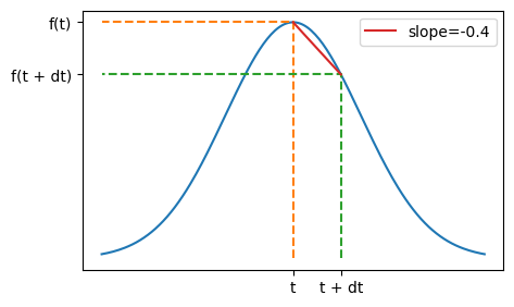
Even more?

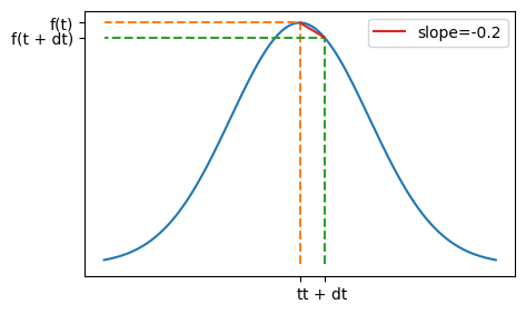
By taking smaller and smaller values of \(\mathrm{d}t\), it becomes clear that we can assign an instantaneous value to the slope at any point \(t\):

\[ \lim_{\mathrm{d}t \to 0} \frac{y(t+\mathrm{d}t) - y(t)}{\mathrm{d}t}. \]

But this is precisely the definition of derivative \(y'(t)\)!

Do you feel more confident?